Conditions and Inference of Linear Regression
Up until know, you should now intuitively that linear regression is the least squares line that minimizes the sum of squared residuals. We can check the conditions for linear regression, by looking at linearity, nearly normal residuals, and constant variability. We also looking for linear regression of categorical variables, and how to make inference on it.
Linearity
The conditions for linearity, is whether you have linear relationship between explanatory and response variables. This is to be expected. Non-linearity algorithm is exist, but beyond the scope of this blog. You might want to check my other blog posts.
We can check the relationship based on scatter plot or residual plots. Take a look at the graph below.
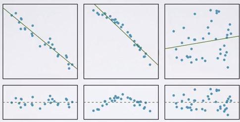
Screenshot taken from Coursera 01:37
The first plot you have good linearity, second plot will give you a more curvy plot, and the third one has highest residual. Not obvious linearity in the third plot.We see residual plots below for the the respective plot. So, how do we make it?
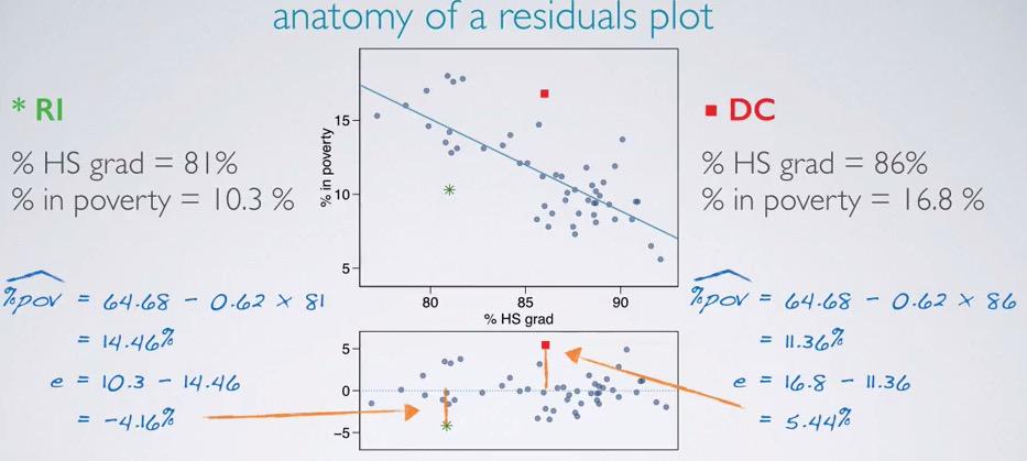
Screenshot taken from Coursera 04:56
We can make the residual plot by plotting the residuals between observed and predicted points. If we predict based on % HS grad, we will have 14.46% for Rhode Island, and 11.36% for DC. We calculate the residuals and have -4.16% for RI (overestimate) and 5.44% for DC(underestimate). Calculate the rest of the data points, and incorporating the linear regression, we will have residual plots.
The ideal residuals is zero, means plot right at the projected line. This is almost zero chance, but nevertheless we want the residuals to be small, scattered around zero. We want the linearity to capture all the pattern in the data, and let scattered around zero would means that it happen by random chance.
Nearly normal residuals
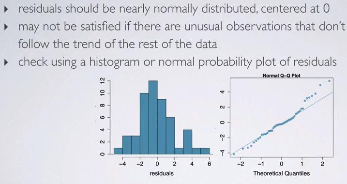
Screenshot taken from Coursera 05:35
The conditions can also be looked at the residuals plot. We can convert all of the predicted and observed to residuals, plot the histogram and see whether it's normally distributed, centered around zero. By looking at plot above, there's few unusual observations, you can also look at the residuals plot, it slightly away from the trend. But this only few observations, so the condition is still met.
Constant Variability
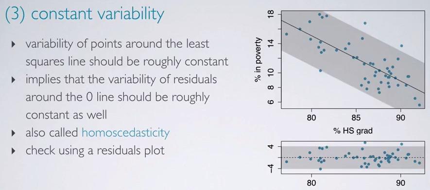
Screenshot taken from Coursera 06:25
The variability for points that scattered around zero in residuals plot is constant. This condition is often called homoscedasticity. By looking at the residuals plot, we can see the variability area (shaded by grey color), constant along x-axis. So you see that as explanatory increases, the variability doesn't get affected.
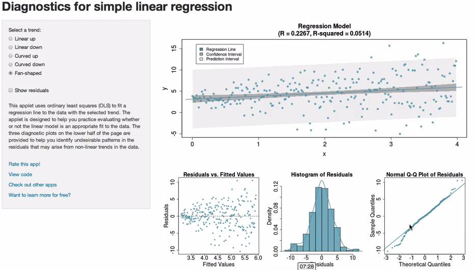
Screenshot taken from Coursera 10:05
Take a look at this link http://bitly.com/slr_diag. Dr Mine Cetinkaya has been kind enough to provide us with this link to play around with kinds of scatter plot and the resulting residuals. You can see that based on the plot in the upper right corner, we can see whether it's constant variability(Plot 1), nearly normal residuals, centered around zero(Plot 2), and linearity(Plot 3).
R Squared
After we checked the conditions of linear regression, we want to meassure how fit our prediction to the observed value. This is where R squared comes into play. This will tell how fit our linear model is. This can be calculated by square the correlation coeffecient. Mathematically speaking because correlation coeffecient is between 0 to 1 and can be negative/positive, R squared is always positive and ranging from 0 to 1.
R squared will tell us the percentage variability explained by the model, and the rest percentage is what's not explained by the model.
Screenshot taken from Coursera 02:53
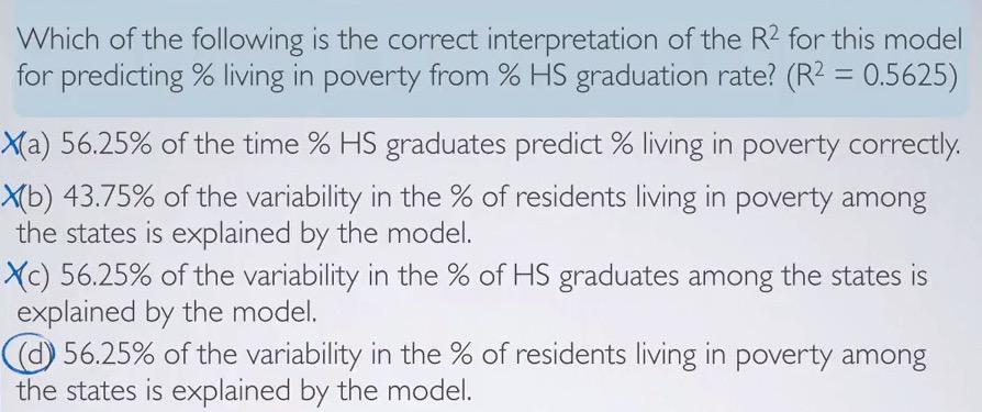
Take a look at the example. We can have R squared by achieving +/- 0.75 in correlation coeffecient.How can we interpret the results in linear regression?
Example A. 56.25% of the time, the prediction will be correct. This would means that 56.25% of the predicted value is fall perfectly in the regression line. This is incorrect. The interpretation is not about the predicting correctly.
Example B. This is talking about the complementary value of R squared and variability of response variable.Although it's more intuitive, this is also incorrect. The complementary value of R Squared is the variability that can't be explained by the model, and not the other way around.
Example C. This explained about the R Squared value and the explanatory variable. This is once again incorrect. We know all about the explanatory variable, and it's meaningless to tell the variability explained by the model.
Example D. This is the one that's correct. We know the R-Squared value is the variability of the response variable that's explained by the model.
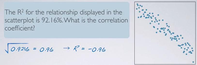
Screenshot taken from Coursera 04:03
In determining the value of correlation coeffecient, you can rely the on the computation software to compute the square root of the given R squared, but then you have to look at the plot to see whether it has positive/negative relationship.
Regression with Categorical Explanatory Variables
Screenshot taken from Coursera 01:44
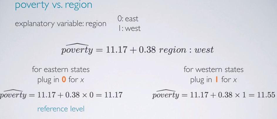
Turns out linear regression can also work with categorical variable as the explanatory. We can have level encoded in the explanatory, and plug in the encoded value, in thise case 0 is east and 1 is west, to the regression formula. An indicator variable is binary categorical variable with two levels(explanatory).
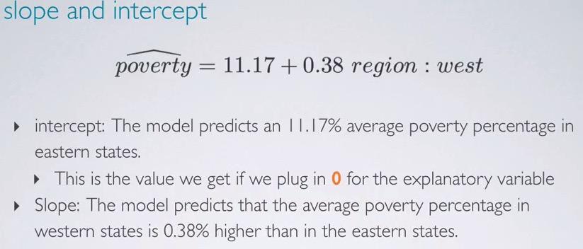
Screenshot taken from Coursera 02:50
So for the the intercept alone, we can predict that the model predicts 11.17% average poverty percentage in eastern states. That is if we plug zero, which the category of west. If we plug one, then the slope will be live, and the model predicts 0.38% higher average than easterns states.
Screenshot taken from Coursera 04:03
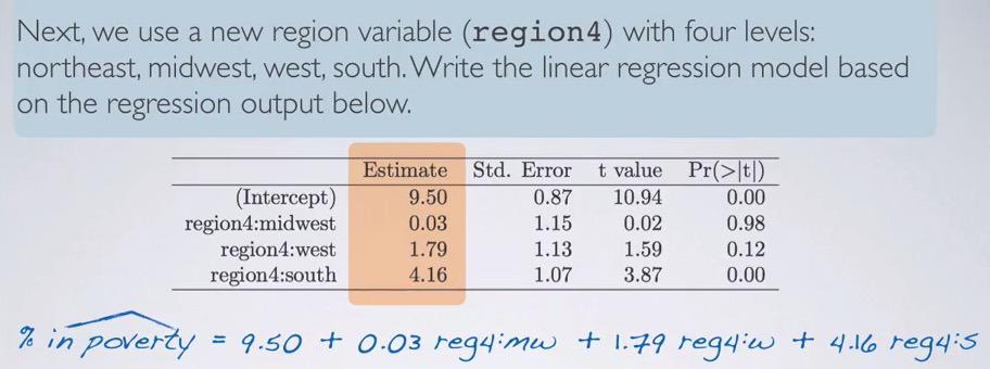
Let's take a look at this example. We ahve 4 levels of categorical variables. We can then make a formula with one intercept and multiple slope, and then just try to make binary 1 level that we focus on otherwise zero.So then what's the reference level? The level that we're trying to set as base comparison? You've seen in the image that midwest,west and south has been set for the slope. So all that's left is northeast, as our intercept.So when we're focusing on the northeast, we set all zero for the slope.
Screenshot taken from Coursera 05:40
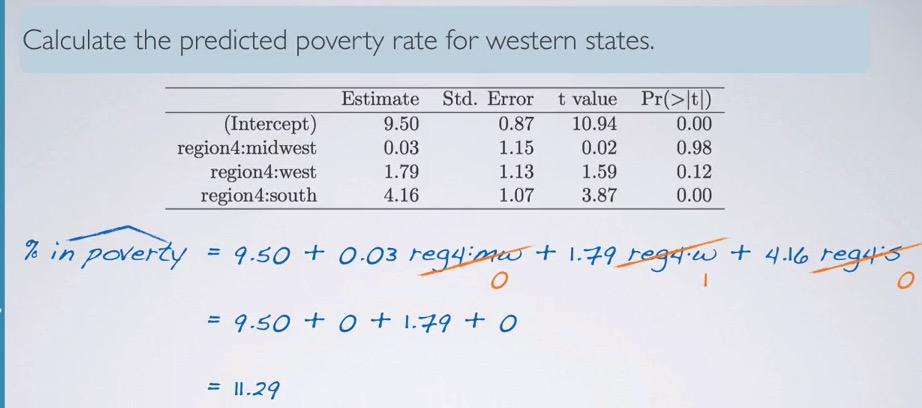
So if we want to focus on west, we can eliminate all the pther slopes so we only have west weight parameters, and the resulting will be 11.29. To interpret this we say, the model predicted 11.29% poverty on average of western state.
Outliers

Screenshot taken from Coursera 01:03
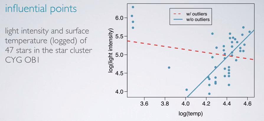
In this section we're going to discuss about outliers. Here without the outliers, the regression line can be horizontal flat. But because outliers, the regression line then change to provide linear regression with outliers included. So you see single outlier will affect our regression line greatly.
Outliers are points that distance away from cluster of points. There are many types of ourliers. Leverage points is points that fall horizontall away from the cluster, so it doesn't affect the slope of the regression, while influential points are high level leverage pints, are points that doesn't fall horizontally, and affect the slope of the line.Usually a better way to test this is plot the points with and without the outliers, and see if the slope line have considerable change.If the slope doesn't change, then the points are leverage, but if it does change, then the points are influential. After detecting the outliers, one must be careful whether to include or exclude the outliers.
Screenshot taken from Coursera 04:41
This is an example of points between light intensity and temperature, by log scale. We can see that with/without outliers, the slope of the line vary greatly. It's depend on what type of finding that you want to focus. If outliers are more interesting thing, then you should include the outliers. But one can not simply join all the trend and outliers. Divide them into two groups, trend and outliers, and make regression line for each of the group. Don't join the model altogether, because it will hurt the model.
So is R squared always get reduced by influential points? No. In some cases, it will affect R squared greatly. So it's not enough to just see R squared and make a decision. You also have make a scatter plot, and detect any influential points that occured. Event one influential points will leverage the slope line.
So leverage points that lies away in horizontal directions, it doesn't change the slope direction. Influential points is the points that change the direction. Determining whether the outlier is leverage/influential, is try to imagine the slope when the outlier is there vs not there.There are have to be a good reason to remove outliers, and if there's level in categorical explanatory that contains few observations but all of it are outliers, this may act as influential points.
Inference
In this section we want to talk about Hypothesis Testing significance, confidence interval, and additional conditions for inference linear regression.
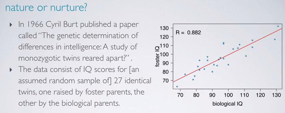
Screenshot taken from Coursera 01:30
Here the study is about different in intelligence when twins raised by one foster and one biological. We can see the from the plot we have positive strong relationship, with correlation coeffecient 0.882
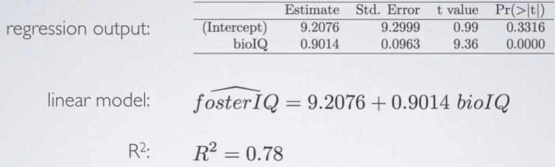
Screenshot taken from Coursera 02:17
In this example, we can say " 78% of foster IQ can be explained by biological IQ". For each 10 points increase in biological twins IQ, we would expect the foster twins IQ to be increase as well by average 9 points. The explanatory is bioIQ and response variable is fosterIQ. twins foster IQ with higher than average are predicted to have biological twins IQ to be higher than average as well.
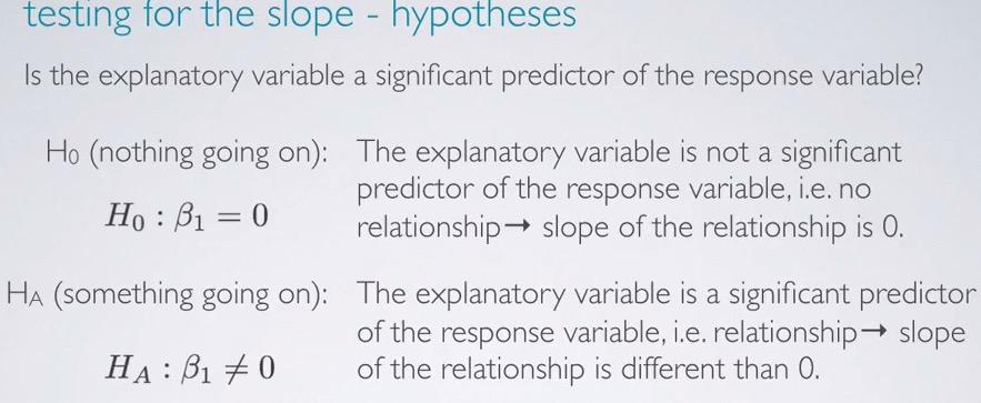
Screenshot taken from Coursera 03:22
For Hypothesis Testing, we want to test that the data provide convincing evidence that biological twin IQ is significant predictor for IQ foster twin.That is hypothesis testing to test whether or not explanatory variable affected the response variable. The skeptical would say no, and the slope is zero, alternative stated otherwise. Recall that B1 is the slope, whereas B0 is null hypothesis.
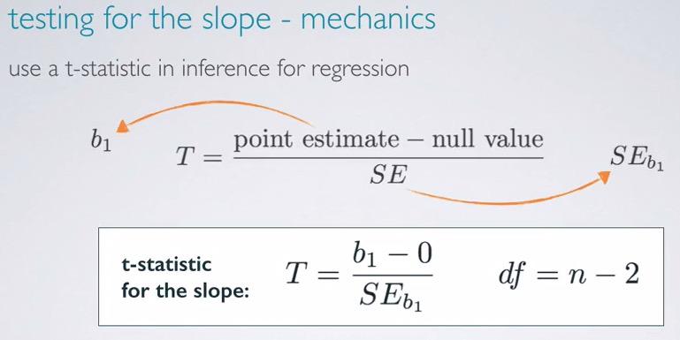
Screenshot taken from Coursera 04:13
Recall that the formulation of t-statistic, we have the calculation for z critical and degree of freedom. So we can plug the formula with slope as point estimate.So why n-2? Remember that for each parameter we calculated, we lose a degree of freedom. Even if you just focus on the slope, it will end up for intercept as well. So we lose two degree of freedom, hence n-2.
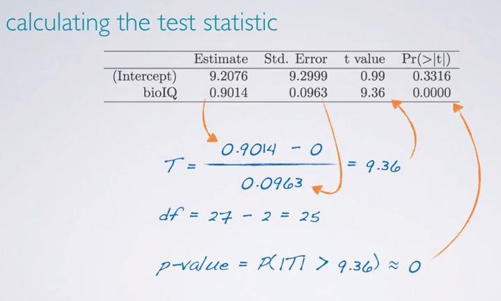
Screenshot taken from Coursera 06:52
Calculating standard error is tedious and very error prone. So here we have already computed table score. Given this we can calculate t-score and get 9.36. As we know this is very huge, and rounding to 4 digits we still get approximate zero. Remember! Even if the computation results to zero, it doesn't mean it equals zero, because p-value can never be zero, it simply just too small even for rounding 4 digits. We can also calculate the intercep and we have almost 1 standard deviation. Remember that hypothesis testing is about two-sided value, so 16% x 2 equals 0.33 like in the computation. So indeed the data provide convincing evidence that biological twin IQ is a significant predictor for foster twin IQ.
Screenshot taken from Coursera 08:54
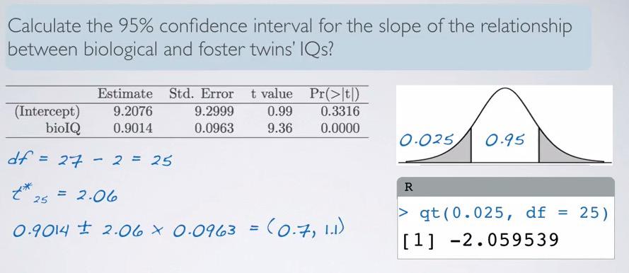
qt(0.025, df = 25)
For confidence interval, we can subtitute the slope and using t-critical for z-score. 95% will results in a little above 1.96, to count t-star for wider interval. Using qt in R we can get our t-critical, which should always be positive. Then the point estimate +/- t_score times standard error, we get the confidence interval. How do we interpret CI? We can say, "We are 95% confident that for each additional point on biological twin IQ, foster twin IQ are expected to be higher by 0.7 to 1.1 points.
Screenshot taken from Coursera 10:43
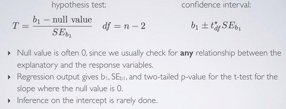
Null value is often zero. Since here we have to catch any relationship between explanatory and response variable. That's also why the null value is zero. On computation, regression output b1,SEb1, two-tailed p-value given null value zero, for the slope. We rarely talk about intercept, because what we often want to infer is the relationship between both variables, which is done by observing the slope.
So conditions must be checked to make inference for linear regression as well. We want's to have random sample (if not often unreliable), less than 10% population, and else to make sure that observations are independent of one another. And if you're already have population data, it's useless to make inference, we only work of what based on the sample data.
Variability Partitioning
Screenshot taken from Coursera 00:54
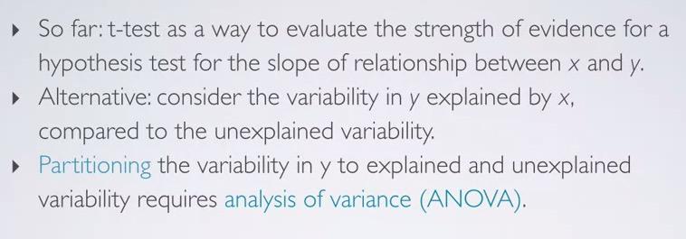
Recall that R squared is about variability of y explained by x. But could it be makes to other way around? Why not unexplained variability dictates y? This requires us to use ANOVA.
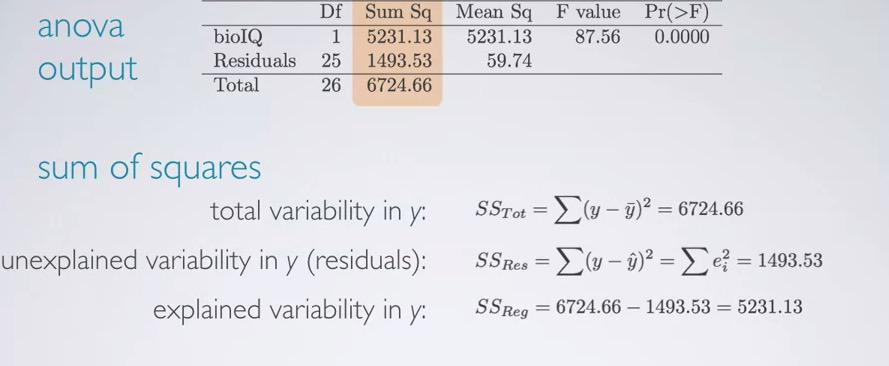
Screenshot taken from Coursera 01:57
Recall that sum of squares total can be calculated by the difference between actual output and the average outputs. So we can sum of squares and have the total difference. We also can calculate sum of squares residuals, with the difference between predicted and the actual output. So we can take explained variability by complements of the residuals.
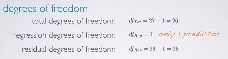
Screenshot taken from Coursera 02:34
For the degree of freedom, we just observing the slope (one parameter) and have 27 samples, so we have 26 total. And because 1 predictor, we get regression df 1. Residuals is just the complement.
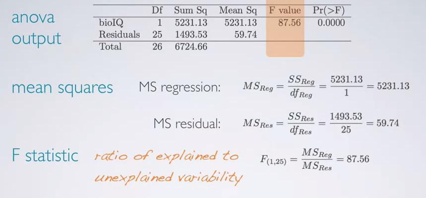
Screenshot taken from Coursera 03:19
Means of squares can be get by SS/df for each regression and residuals. Recall that F-statistic is ratio of explained to unexplained variability. Which means that as we get higher F score, we get a good estimate.
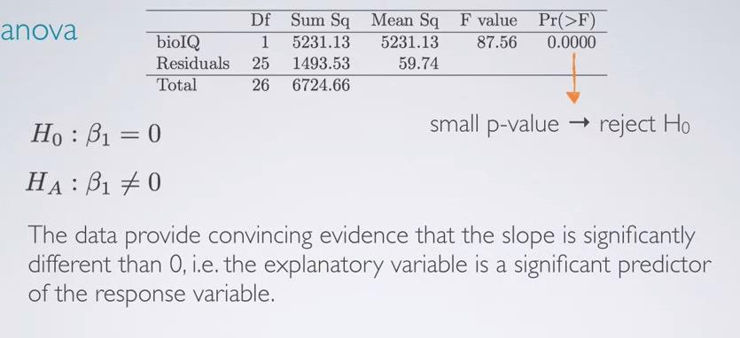
Screenshot taken from Coursera 04:02
For hypothesis testing, the p-value is approximate zero. Hence we reject the null hypothesis and conclude the data provide convincing evidence that the slope is significantly different than zero(we said significantly, if it pass the significance level), i.e explanatory variable is a significant predictor of the response variable.
Screenshot taken from Coursera 05:03
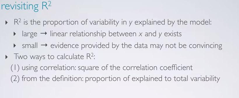
R squared is the proportion of variability y explained by the model. Larger value will yield larger proportion of y variability y explained by the model. Small will means the evidence is not convincing to be significant predictor. Two ways to calculate R squared, square the correlation coeffecient, or proportion of explained ratio to total variability, as calculated by ANOVA. We can validate R squared using both methods.
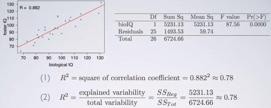
Screenshot taken from Coursera 05:46
Using both models we achieved roughly 78%. So 78% of twin foster IQ (response variable) can be explained by the model, in other words, twin biological IQ (explanatory variable).We want to keep R squared to be approach 1, because that is the ideal model, which can predict all the y output.
In summary, we can use t-test and the resulting p-value to determine whether the indicator variable, the predictor, is sifnificant predictor or not. Regression output computed by the software always yields two-sided p-value given null hypothesis zero. We lose two degree freedom to account for intercept and slope parameters.
Why we rarely have HT for intercept? Because the intercept point may outside the realm of data and usually an extrapolation. In other words, extrapolation means predicting for any given value of x outside the realm of data.
REFERENCES:
Dr. Mine Çetinkaya-Rundel, Cousera