Frequentist vs. Bayesian Approach
In this blog we're going to discuss about frequentist approach that use p-value, vs bayesian approach that use posterior.
Screenshot taken from Coursera 01:04
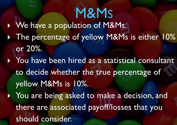
The study will help us make a comparison of frequentist vs bayesian approach. We have a population, and your task is to test whether the yellow is whether 10% or not.
Screenshot taken from Coursera 01:52
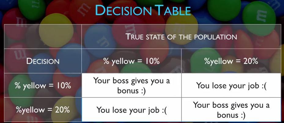
Then from the study, you make a decision table. If your decision is right, you're going to get a bonus, otherwise you lose a job.
Screenshot taken from Coursera 02:26
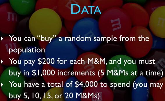
Then you're presented the money and the cost to gather the data. Remember, often it's pretty costly to get more data. So this example representing that condition.
Using frequentist approach, you're going to use hypothesis testing. To set the hypothesis:
- H0 : 10% yellow M&Ms
- HA : 20% yellow M&Ms
Using test statistic, because it's talking about the proportion, is the number of yellow observed in the sample. The p-value is calculating the probability of this many or more yellow M&M in the sample that you have buy, given the null hypothesis test. You might want to ask this, "If I have bought 3 times and observe all the p-value, can I predict what is the p-value for the fourth time?"
So how many sample that you think you would buy? 5,10,15,20? Recall that if you fail to predict the p-value, you would lose your job. But if you buy large sample size, it will be very costly. The decision is how to get the right sample size, that's enough to make it practically significant.
Let's choose 5 for this state. If some of you have known bootstrapping, this is one of the most important technique to engineer a new sample. In hypothesis testing, you're collecting the data, build test statistic, p-value, and compare it to significance level. The next question then become, what is significance level for this problem? Recall that significance level is all about type 1 error, rejecting the null hypothesis when the null hypothesis is true.
So which level should you choose? Using higher significance level, you can have a type 2 error rate. But using smaller alpha, can get you miss any true significant p-value. For this case, we stick with 5% significance level.
With sample size this small, we can use binomial distribution.Because we set 10% as our null hypothesis, we set the probability of success 10%. Recall that null hypothesis is a null value for true population,hence the proportion is equal the probability of success. Suppose we have yellow (among 4 other colors) once.
p-value = P(1 or more yellows | n=5, p = 10%)Since we're observing the probability of at least 1, and there are only two chances, whether it's yellow or not, we can simplify this calculation as,
P(k>=1) = 1 - P(none yellows)
The complement probability is 0.9, then
P(k>=1) = 1 - (0.9)^5 = 0.41
The result is 0.41, our p-value is greater than the significance level, we failed to reject the null hypothesis.
Since the sample size is indeed small, and because of that, we want to increase our sample size to 10. Then for the 10 draws, we get two yellows. The p-value is then
p-value = P(2 or more yellows | n=10,p=10%)
Since this is getting too complicated(we can calculate the probability of 2,3,4..10, or 1-(k=0+k=1)), we can use R.
sum(dbinom(2:10,10,0.1))
Again, based on this p-value, we fail to reject the null hypothesis.
How about the 15 sample size? Again when doing 15 draws, we get 3 yellow. So,
p-value = P(3 or more yellows | n=15, p = 10%)Using R,
sum(dbinom(3:15,15,0.1))
Again we failed to reject the null hypothesis.
For the sake of the argument, we use 20 sample size, and have 2 yellows in 20 draw. Again we set our binomial,
p-value = P(4 or more yellows | n=20,p=10%)sum(dbinom(4:20,20,0.1))
And then, once again, we failed to reject the null hypothesis.
Screenshot taken from Coursera 14:33
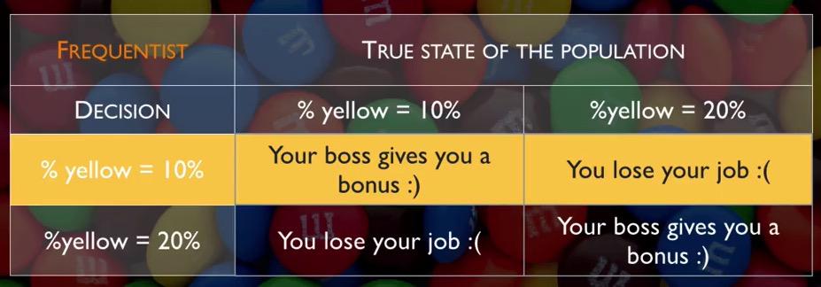
If we're looking at the possibilities earlier(1 out of 5, 2 out of 10, 3 out of 15, and 4 out of 20), we know that the proportion is actually 20%. Since we failed to reject our null hypothesis, we would lose our job.So you see, it's important to see from looking at the problem.
Screenshot taken from Coursera 15:30
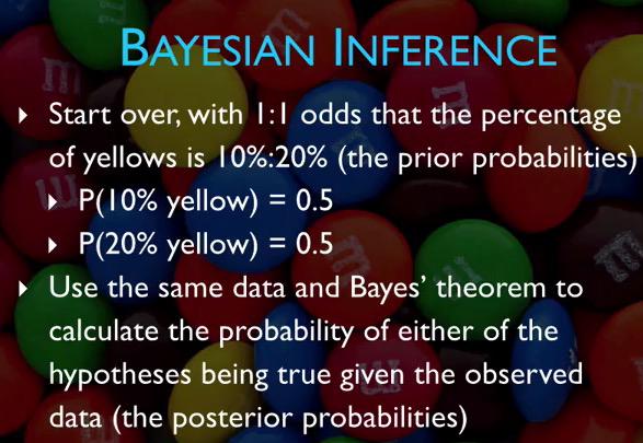
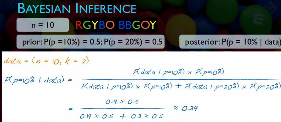
Now let's use bayessian approach. Again, only two conditional probabilities.You can either have 10% or 20%. Since we don't how is the true population, we make a fair judgement 50:50. In Bayes this is our prior probability. As you recall in Bayes, we can be presented with the data, calculate the posterior, make that as an input of next data, calculate the posterior and keep doing that.So the p-value in bayesian is the probality that given the observed data, what are th posterior probability.
Screenshot taken from Coursera 17:16
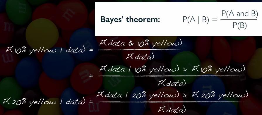
So we can calculate the probability of 10% given data. This is what Bayesian can solve. We can use Bayes to calculate like the one in the examples. Recall that in Bayes, we have
P(A and B) = P(B and A), if A and B are dependent.
P(A|B) * P(B) = P(B|A) * P(A)
We subtitute the equation like the one in the example. Since there either 10% or 20%, the probability of 20% is the complement of 10% yellow.
dbinom(1,5,0.2)
Screenshot taken from Coursera 20:18
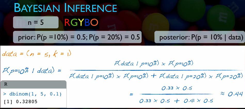
dbinom(1,5,0.1)
dbinom(1,5,0.2)
Once again, since we only have two conditions in our probability space, and we're observing the exact successes for n trial, we can use dbinom function. Recall that we have 1 yellow in our first trial. We calculate the Bayesian as observing the probability of 10% given the data. And by calculating the probability of data, what is the probability that we have 10% yellow or 20% yellow given the data. Since we have an or in probability, we join by addition. In dbinom we can calcute the probability of k success, given n trial, knowing the probability of success. We can use P(data | 10%) with dbinom in R. So we're calculating P(data|10%) is 0.33 and P(data|20%) is 0.41. We incorporate the formula, and have 0.44.
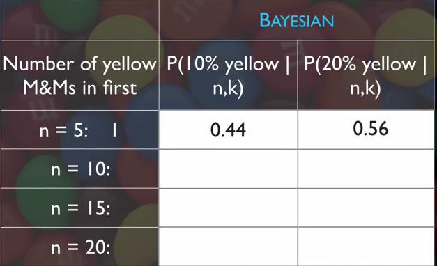
Screenshot taken from Coursera 21:40
You may want to mark your results in the table. Since 20% yellow is the complement probability of 10%, we take it 0.56 for the 20%. And we repeat our process for 10,15,20.
Screenshot taken from Coursera 23:05
dbinom(2,10,0.1)
dbinom(2,10,0.2)
for 10 value, we can get 0.39 for P(10%|data). And the complement for 20% is 0.61
p_data_10 = dbinom(3,15,0.1) * 0.5
p_data_20 = dbinom(3,15,0.2) * 0.5

p_data_10/(p_data_10+p_data_20)
So we have 0.34 for P(10%|data) and for the complement of 20%, we have 0.66. That is our posterior probability of step 3.
p_data_10 = dbinom(4,20,0.1) * 0.5
p_data_20 = dbinom(4,20,0.2) * 0.5

p_data_10/(p_data_10+p_data_20)
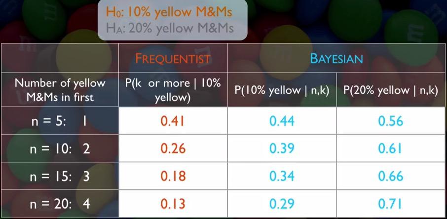
Finally, for 20 M&M we have 0.29 for 10% and the complement 0.71 for 20%. Let's take a look at the overall table, all 4 steps of frequentist vs bayesian approach.
Screenshot taken from Coursera 27:31
The frequentist approach, p-value makes HT failed to reject, and keep siding with 10%. On the other hand, Bayesian consistently prefer 20%. So there's two contradicting results on two approach. Which is right? Since you know that 20% is the true population, Bayesian is the winning side. Indeed sometimes two approach could yield slightly different result.
Recall that in Bayesian, you'll always update prior according to your posterior. Earlier, we don't update our prior. It keeps at constant 0.5.How about we keep updating prior based on resulted posterior? You could also using Bayesian approach like this
p_data_10 = dbinom(1,5,0.1) * 0.5
p_data_20 = dbinom(1,5,0.2) * 0.5

p_10 = p_data_10/(p_data_10+p_data_20)
c(p_10,1-p_10)
p_data_10 = dbinom(2,10,0.1) * 0.44
p_data_20 = dbinom(2,10,0.2) * 0.56

p_10 = p_data_10/(p_data_10+p_data_20)
c(p_10,1-p_10)
p_data_10 = dbinom(3,15,0.1) * 0.34
p_data_20 = dbinom(3,15,0.2) * 0.66

p_10 = p_data_10/(p_data_10+p_data_20)
c(p_10,1-p_10)
p_data_10 = dbinom(4,20,0.1) * 0.21
p_data_20 = dbinom(4,20,0.2) * 0.79

p_10 = p_data_10/(p_data_10+p_data_20)
c(p_10,1-p_10)
So there you go, using Bayesian approach, you get 0.1, which is near to 0.13 frequentist.
REFERENCES:
Dr. Mine Çetinkaya-Rundel, Cousera