Hypothesis Testing
Snapshot taken from Coursera 04:09
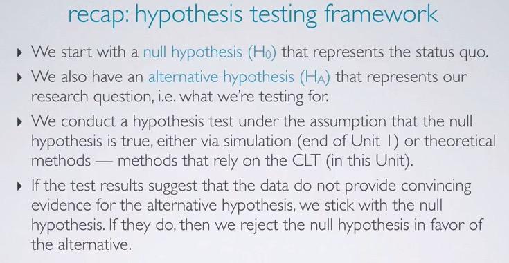
Earlier in my blog post, we have learn about hypothesis testing. Based on the difference of 30% in female vs male being promoted, we want to know if the difference makes two variable independent vs dependent. The Null Hypothesis said that is due to chance. The alternative said, there's dependant variable and some relationship. Using simulation earlier we know that achieving 0.3 is very rare using simulation. If there's no strong evidence, we stick to the Null Hypothesis, but if we do we reject the Null Hypothesis in favor of the alternative. We can do this by using CLT, like in the Kloud score example.
In a way, Hypothesis Testing is similar to what we do in court trial. There's skeptical that judge whether the one in court is guilty or not guilty. The judge will pressume that the man is innocent, until strong evidence prove that the judge reject the innocent and set him guilty. The court is not about the evidence, it's about whether it reject, or fail to reject the innocent.
Snapshot taken from Coursera 01:08
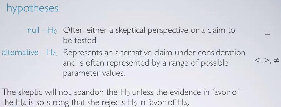
Null Hypothesis is skeptical claims that there's no difference between two variable, sometime denote by equal value. In above cases,
P(female) = P(male)
Alternative Hypothesis claim theres difference between two variables, and represented by range of values (>,<,$\neq$)
P(female) $\neq$ P(male)
The skeptic will keep sided with Null Hypothesis until there's strong evidence to reject it.
So HT is all about population parameter, because it's often not defined. There's no point in testing sample statistics. H0 is about the skeptical, that is there's no difference, and set null value to be the value of H0. The HA on the other hand is state that there is different, $\neq$ two sided, or less/greater than, one sided.
Snapshot taken from Coursera 03:11
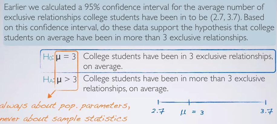
The hypothesis testing is always the population parameters $\mu$ and not sample statistics $\bar{x}$. It will always be that way. This synchronize with CI that always concern about the population parameters. Hypothesis testing is not about sample, because we already know the sample, and we want to guess the population parameters. In this case, when we know 3 is in the range of interval, we can't reject the Null Hypothesis.
Snapshot taken from Coursera 05:19
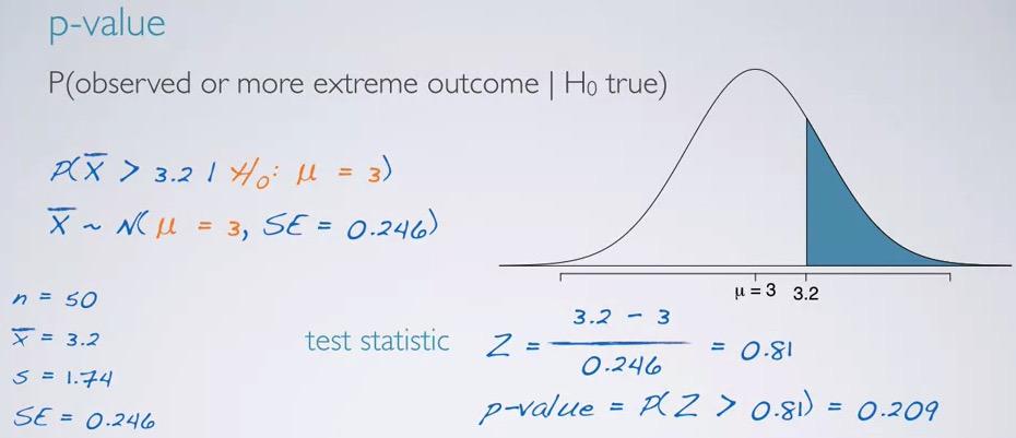
Pay attention to what p-value described above. The p-value is a conditional probability that given null hypothesis is true, what is the probability of at least as extreme as observed outcome.
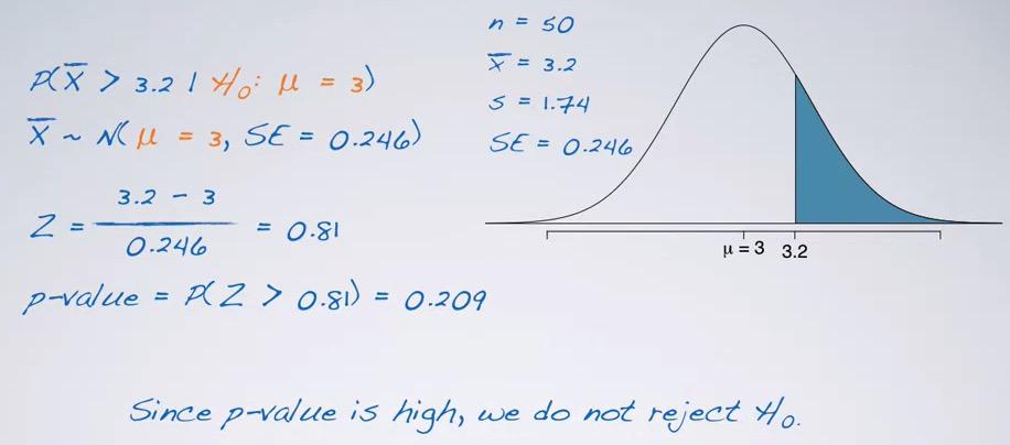
Suppose we are asked the probability of average more than 3.2. p-value is the probability of observed point estimate at least as extreme or more given the Null Hypothesis. Under the assumption that null hypothesis is true, we can use mu as our basis, and compute the Z-score. Attaining z-score is a matter of calculating the distance from mu divided by standard deviation.Z-score is often called test statistic, where we want to test our statistic parameter 3.2. Using z-table we get p-value of 0.209. In R
%R pnorm(3.2,mean=3,sd=0.246,lower.tail=F)
Snapshot taken from Coursera 06:03
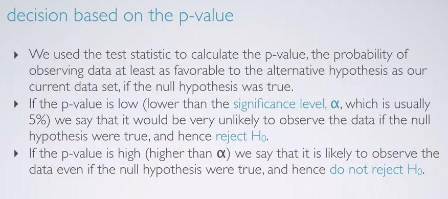
the p-value is used to calculate the extreme condition where at the very least sided with alternative under the condition of null hypothesis is true. If the p-value is low, lower than threshold 5%(commonly used), $\alpha$, we can reject our null hypothesis. But even under null hypothesis is true the p-value is higher then $\alpha$, then we stick to Null Hypothesis.
Snapshot taken from Coursera 06:59
So calculating all those, we have 20.9%, which is larger than 5%. We know that under the condition that our Null Hypothesis(average = 3) true, the p-value makes we can't reject Null Hypothesis in favor of the alternative (average >3.2).So we stick to the Null Hypothesis.
Snapshot taken from Coursera 07:44
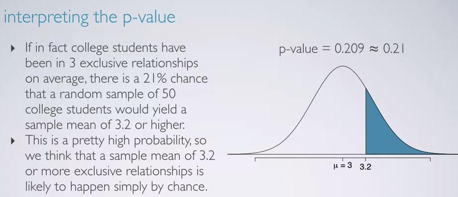
Remember the p-value is always take assumption that Null Hypothesis is true. Under the assumption of that, there's two condition. 21% chance average of 3.2 or higher, or average of 3.2 or higher is due to chance.
Snapshot taken from Coursera 08:14
When talking about sampling distribution, 3.2 means that average of our sample is due to chance or sampling variability. Based on data that we have, it doesn't provide convincing evidence that the average is higher than 3 relationships.
Snapshot taken from Coursera 08:54
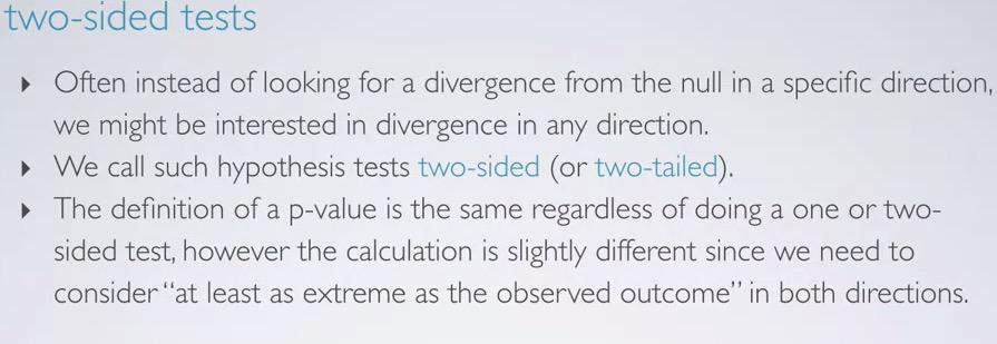
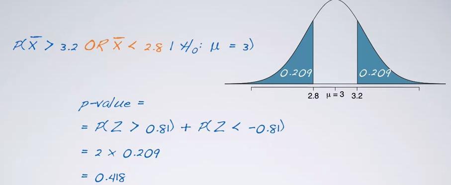
The two-sided will be the same as one-sided, except that it takes range, a divergence instead of one. So we have to have substracting in two sided if we want to know the range of value in between, or takes sum over two cut tail, if we search for less than or greater than.
Snapshot taken from Coursera 10:13
%R pnorm(3.2,mean=3,sd=0.246,lower.tail=F) + pnorm(2.8,mean=3,sd=0.246)
Snapshot taken from Coursera 14:01
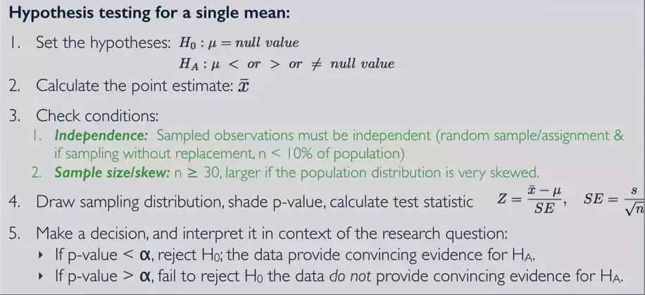
So this is the complete steps of Hypothesis Testing Framework.
- Remember that the Hypothesis is always about the population parameter, where NH = null value, and AH $\neq$ null value.
- Calculate the sample statistics, if we want to estimate the mean of population, we calculate mean sample and set that as point estimate.
- Check that the distribution is normal/skew, check that we indeed have random sample in our sample by following condition 2. Plot boxplot or histogram to see the shape of your sample distribution.
- Next, draw sampling distribution, shaded the cut off value to get better understanding, and calculate test statistics.
- Finally, after making calculation, be sure to interpret the data based on the research question.
Hypothesis Testing(mean) example
Snapshot taken from Coursera 02:19
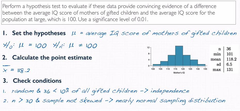
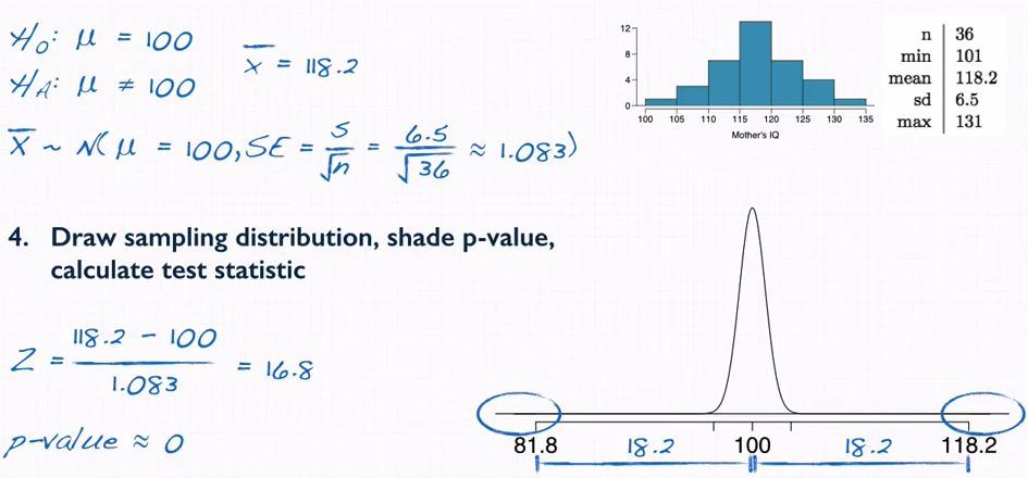
So now we're taking one problem, and follow the steps of HTF. This example also stated that sample collected by gathering thirty-six mother that has gifted children, testing the children when they achieved age of four.
- We set the hypothesis, from the question we know that the there's two competing events, one true average of IQ mother of gifted children vs true average IQ population. We then know that $\mu$ is 100.
- We check the point estimate, since we're talking about average here, we calculate $\bar{x}$ and that is 118.2
- We check the condition. Other than less than 10% population, we know that the researcher sample one mother, therefore a mother should be independent for another mother that has 4 year old children. We also now the shape of the distribution is nearly normal, so more than 30 should be enough.Following this condition, we can expect our sampling distribution is normal.
Snapshot taken from Coursera 04:26
Next we do step 4.
By knowing $\bar{x}$ and the sample size, we can compute the standard error. When we draw the sampling distribution. We know that the width of the distribution is very skinny. calculating The Z-score what we get is 16.8. So 16.8 standard deviation away from the mean! This is actually very far.Because we're doing two side tail, we multiply by 2. Doing R, the p-value we get is
%%R

pnorm(118.2, mean=100,sd=1.083,lower.tail=118.2 < 100) * 2
We get very low probability approximately zero. In this case we're reject Null Hypothesis, that stated true average of IQ mother gifted children vs IQ population is not due to chance. Thus we reject it and favor the alternative hypothesis, that stated it's not the same.Therefore we provide strong evidence that there is a difference between average of IQ mother of gifted children and average IQ population at large. And that's step 5, Make a decision and interpret based on context research question. Because we reject the null hypothesis, the interval of IQ mother sample is not capturing true average of IQ population.
Snapshot taken from Coursera 06:55
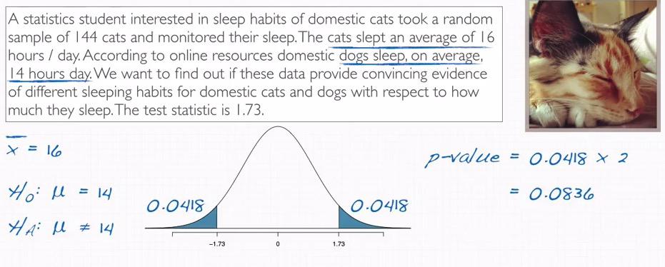
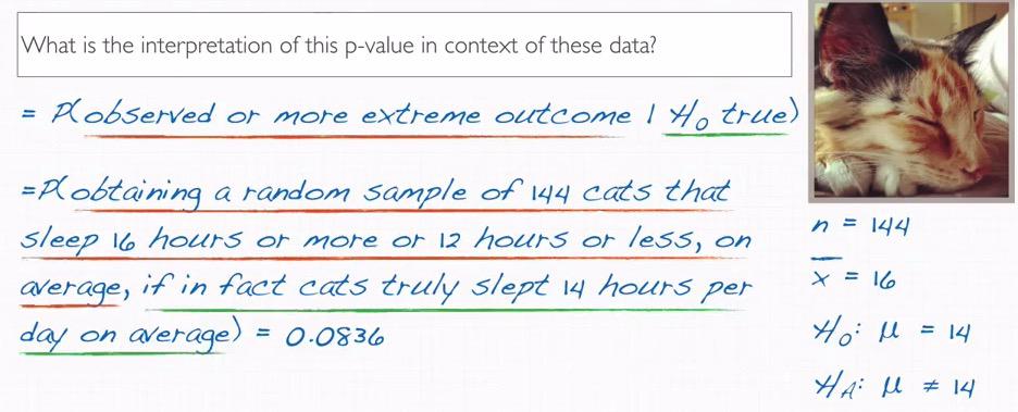
Next for new problem, we want to provide an evidence of difference between cat sleep and dog sleep.Remember that test-statistics == Z value. And thus we can directly calculate two-tailed t-test equals 0.0836. The test statistics is gathered that given the dog is slept average of 14 hours/day, what are the probability of the cat, in the sample which slept 16 hours a day.
Snapshot taken from Coursera 09:19
Because this is two-tailed test, and 16 is 2 more from the mean, 14, we can also say 2 less than the mean, which is 12. So two-tailed p-value intrepret as the probability of extreme random sample 16 hours or more or 12 hours or less, is 0.083. Remember the p-value can be interpret two things. One is that either we keep or reject the null hypothesis. Second we can state the probability(p-value) of at least as extreme or more(2 hours) from the observed value, 14 hours a day.So the probability that we get from our sample is 0.0836.
Inference for other estimators
So far we've learned about doing inference that we gather from sample, like sample mean and sample standard deviation infer the unknown population mean. Turns out HT isn't just that, next we begin to open a variety of estimate within HT and confidence interval.
Snapshot taken from Coursera 01:28
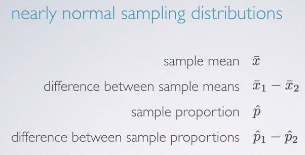
So other than mean, we also can calculate the proportion. Remember that proportion is between 0 to 1. And not only mean and sample of one sample, but also the difference between two sample, for example two sample group.
Snapshot taken from Coursera 02:13
Fortunately, based on CLT, sampling distribution always gives aprroximately normal distribution and centered around true mean population, or other point estimate that just listed. Therefore, the it will give unbiased estimate from the true population parameter.
So remember again, confidence interval for nearly normal point estimates is:
$$ pointestimate \pm z* x SE$$
Note that for all confidence interval, we always start with point estimate, and give plus or minus based on that. The plus minus difference will be our margin of error and it incorporates z-star, assume that our sampling distribution is nearly normal. Remember that for CI we must follow the normal condition and unbiased. CI is always applicable to all kind of point estimate, but Standard Error has different calculations for each of them. So remember, all requirements and the calculations are the same, except the calculations about SE.
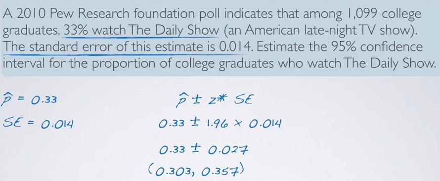
Snapshot taken from Coursera 05:28
In this problem, the standard error has been given. Here we see that it know has point estimate, proportion denoted as $\hat{p}$ , confidence level, and standard error. Plug all those we have our interval.
HTF is also applicable, same as CI but still follow the conditions unbiased and normal shape distribution. The formula is:
$$Z = \frac{pointestimate - nullvalue}{SE}$$
Consider following example
Snapshot taken from Coursera 08:23
Here we calculate the difference of sample mean between two group. As before we convert the problem into our HTF.
- Set the Hypothesis. Here we are asked to provide strong evidence that men and women has different BF%. So we set H0 : $\mu$ men = $\mu$ women. The alternative, HA: $\mu$ men $\neq$ $\mu$ women
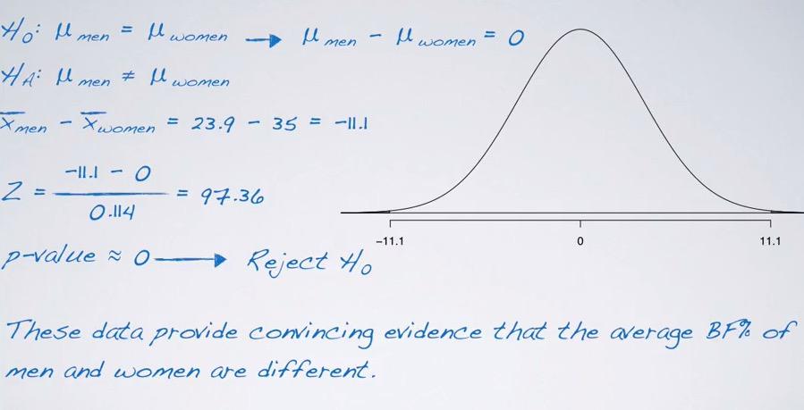
- Next we calculate the point estimate. In this case the point estimate is the difference of sample mean between two group, hence simple substracting $$\bar{x} men - \bar{x} women = 23.9-35 = -11.1$$
- Check the conditions. we already given information that the distribution of point estimate is nearly normal. In Addition, we also know that the it's national survey. Hence we expect to safe because they already randomly sample and have independent samples.
Snapshot taken from Coursera 10:03
So if we plot it into sampling distribution, where's it has centered? Since the sampling distribution centered around the null value we observe each of mean female and male. Since they're not given, that's not matter. Because under the assumption that both are same value, we can expect the differece is 0, so it will centered around 0. We have the cut-off value of -11.1 the difference, and have two-sided t-test. When draw the distribution and shade the p-value, it's really small. Remember that we're looking the difference, hence it's exclusive within distribution. So more than 11.1 or less than -11.1. Calculating the Z-score we got 97.36. So far standard deviation away from the mean, which mean p-value is bound to be zero. Thus we reject the null hypothesis, and doing step 5, we intepret it as the statement These data provide strong evidence that there is a different between true average BF% of men vs women population.
Remember that CI and HT is agree with each other. CI always have interval that capture null value in HT. We will discuss this in the next section.
REFERENCES: