High to Low Level Metrics A/B Testing
Earlier when choosing metrics, we go through 3 steps: Defining the metrics, build intuition about our data and our system, and finally characterizing the metrics. We have talked about defining turn high level concept into metrics that we want to measure. Also talking about filtering any potential bias. This blog discuss how to turn high level concept of metrics into lower more technical metrics. Then we create summary metrics in form of statistics to build intuition. Specifically, we discuss about measures of center of summary statistic in the metric for experiments.
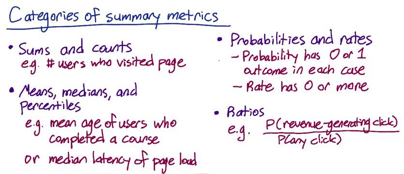
Screenshot taken from Udacity, A/B Testing, Summary Metrics Example
In general, there are 4 categories that we need to keep in mind. The first one is easy, when talking about number of users, we want to see the counts of users who visited the page. You can track it over time series (week,day,year). The second one is when you plot the distribution of the metric by histogram. Is the distribution is normal, you can use mean, and median. But if it's funnier, you can use percentile. It also important to recall what are the changes that you care about. There are probability and rates, which is good for computing like average or sum. Finally, ratios, which is useful for a lot of business context, but also hard to measure.
When evaluating summary metrics, there are two things that we should do. First we test the metrics by sensitivity and robustness. Our point estimate must be sensitive, in the changes that we care about, and robust, in changes that we don't care about. For example we choose percentile as our point estimates. If you use experiments, whether is't running or past experiments, you want to check that changes in percentile that you choose is makes sense.
Second we test the distribution of metric (by looking at histogram or retrospective analysis). If you use retrospective analysis using log, you want to see changes you make based on your log fit in conjunction to metrics that you want to count.
Sensitivity and Robustness
Screenshot taken from Udacity, A/B Testing, Summary Metrics Example
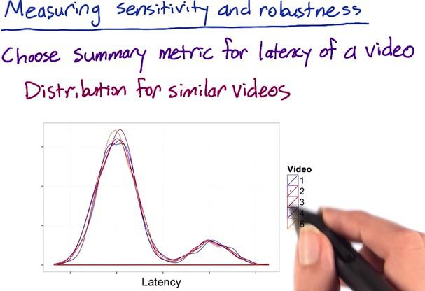
Suppose we take video latency from Audacity MOOC course. We take 5 video (assume all comparable), and using density distribution to plot the count of the latency. We use retrospective analysis and experiments to see which changes fit in percentile. With retrospective anlysis using log, we plot in histogram gives us bimodal distribution, people who have greater internet access, and people who have shorter internet access. The goal of this experiments, is whether to see which resolution should people start from. Is it from high res or low res.
Screenshot taken from Udacity, A/B Testing, Summary Metrics Example
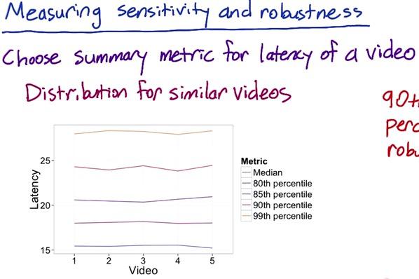
Suppose we have 5 different videos and have a point estimate (median and percentiles) to summarize video latency across people. These latencies are shown as bimodal distribution in our previous picture. When looking at this plot, we see that 90th and 99th percentile show zig-zag line compared to the rest of the percentiles, which tells us is not consistent. We don't even apply any changes at all (remember this is just retrospective analysis), and here we see 90th and 99th are not robust to changes that we don't even care. For this reason, we exclude 90th and 99th percentile.
Screenshot taken from Udacity, A/B Testing, Summary Metrics Example
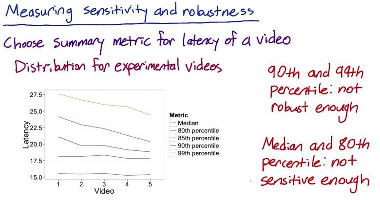
Next we want to if these summary metrics sensitive to changes that we care, we change our resolution to low resolution using experiments. After that we plot the percentiles the same as we test the robustness. We see that after applying some changes, median and 80th percentile is stabil, but the rest of percentiles is having an effect after we apply changes. Stability of median and 80th percentile on the plot above after we apply some changes, mean that these percentiles is not sensitive enough to changes that we even care about. So while 90th and 99th are not robust, median and 80th percentile are not sensitive. Which leave us 85th as the only one summary metrics that sensitive and robust.
There are two ways to compare the difference of your summary metrics between experiment and control groups. First is absolute difference, where you just substract the difference of both groups. The second is relative difference, like ratio difference or percent changes. Absolute difference is useful when you have little experiments, or you just starting out. But it's not so useful if you run your experiments across period of time. For example number difference of conversion users in summer maybe different with number of difference in winter. This is where relative difference such as percent changes shines, where it could only use one practical significance boundary span over time. If you have lots of experiments, relative difference is also useful. The downside of using relative difference is often it's not well behave and not very intuitive. So for starting point, it's good to use absolute difference and go from there.
Disclaimer:
This blog is originally created as an online personal notebook, and the materials are not mine. Take the material as is. If you like this blog and or you think any of the material is a bit misleading and want to learn more, please visit the original sources at reference link below.
References:
- Diane Tang and Carrie Grimes. Udacity