t-distribution and ANOVA
Big Data is the terms that comes a lot in the data scientist. Is big data equals accuracy? Not necessarily.We've seen enough examples where the data is small, but enough for many statistician to infer from the data. In this blog, we will discuss how we're dealing in small sample size vs large sample size and make inference based on it.
Recall that for all observations that independent and population distribution is not extremely skewed, large size will ensure that:
- The sampling distribution will be nearly normal
- We have smaller standard of error, hence more reliable estimate.
Recall also that for CLT, As long as the population distribution is normal, the sampling distribution will also be normal with any given size.
While that might be useful information, but as long as we have small sample size, we can't infer the distribution of population. From normal distribution of population, sample size of 10 might not be normal enough compared to 1000 sample size. Therefore one must be careful enough to observe the samples. It doesn't good enough to know shape of distribution of the sample size. Ask yourself a question about the data itself. Make an intuition about the distribution of population that you concern. What is the modality, is it symmetric, are you sure that outliers are rare. This will comes in handy and always be suspicious about small sample size.If this is your problem, then you might want to try t-distribution.
t-distribution
Screenshot taken from Coursera 06:03
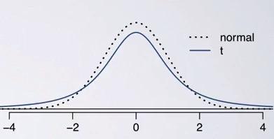
t-distribution address the problem where you have small sample size and you want to meassure the uncertainty of your standard error estimate. You know that standard error consist of sample size and standard deviation of your sample. But if you have small sample size, your standard deviation might be unrealiable, hence unrealiable standard error.
This is the case where we use t-distribution. As you can see, t-distribution has similar look to normal distribution, but with a lower top and thicker tails than normal. Thicker tails here is an additional help to your sample, to make even greater variability estimate of your data.This will help to reduce of a less reliable estimate of standard error in your sampling distribuion.That The observations in t-distribution will be expected within 2 standard deviation from the mean.
Screenshot taken from Coursera 07:13
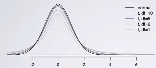
As like normal distribution, t-distribution will be centered at 0. But it comes with additional parameter(aside of mean and standard deviaiton), which is df, stands for degree of freedom, that determines the thickness of t-distribution. The higher df, the closer it is to normal distribution.Smaller df will result in longer tails, as you can see that higher than 2 standard deviaiton will give you 7% area of both side(wider variability, df=10),and a little more than 5%, on df 50.
Instead of z-statistics that we always calculate in CLT, we use t-statistics. But that just a naming convention. All still the same with normal distribution. calculation for t-statistics is the same as z-statistics(z-score), and the p-value is also the same, for both one sided and two-sided (depending on p-value).
t-test is used for inference that CLT can't further ado. This include where the population standard deviation $\sigma$ is unknown and sample size is less than 30.
Screenshot taken from Coursera 12:44
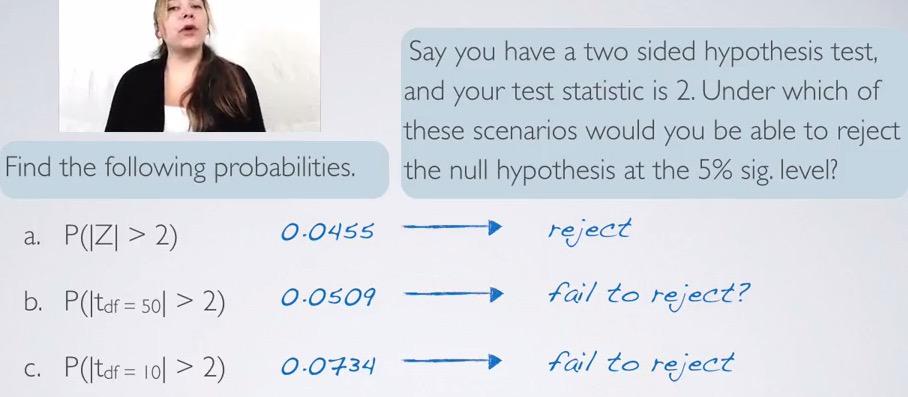
Here is the cases where we have Hypothesis testing for calculating the p-value for all two standard deviations aways in normal distribution, t-distribution with df=50, and df=10. As you can see, being normal distribution, less than 5% will reject, tdf=50 is close to 5%, it depends on the situation whether we want to reject it or not, and finally tdf=10 which clear fail to reject the null hypothesis. What does this means? For hypothesis testing, it's harder to reject null hypothesis under t-distribution rather than normal distribution. For sample size less than 30, t-test making it stronger threshold rather than t-test.
As we note earlier, lower df result in greater flexibility, and thus making it more sided with null hypothesis. df is directly correlated with sample size, where you have low sample size, you also want to have lower df, and that means greater flexibility.
t-distribution is found by William Gosset, Head of Experimental Guinnes at 1900, and produce the paper which the foundations of t-test under the fake name, student. Hence called, student's t.
Let's take one example using t-test
Screenshot taken from Coursera 02:20
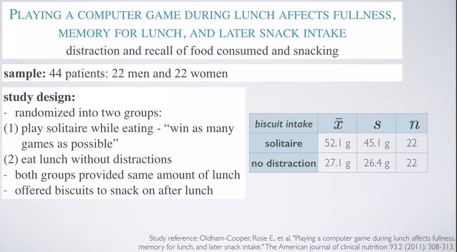
Study taken for 44 patients 22 men vs women (less than 30) and each divided into treatment and control group (blocking).
Screenshot taken from Coursera 04:34
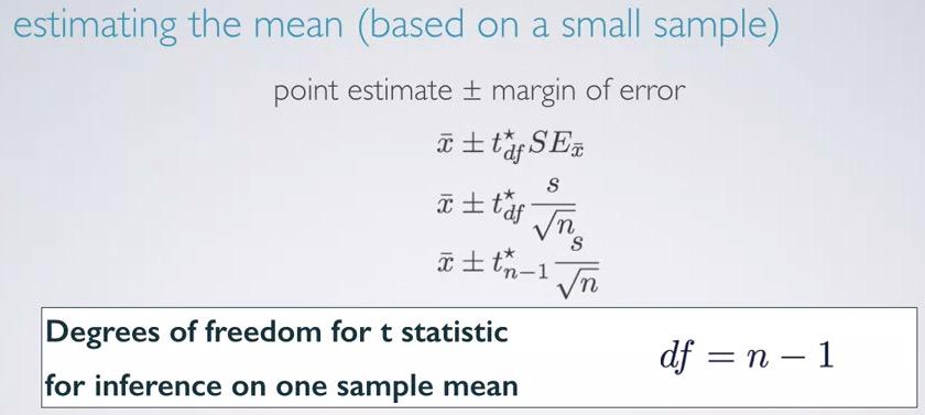
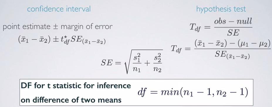
here we have usual calculating confidence interval formula. This must be familliar to you that already have understanding about confidence interval. The df is simply n-1. Why? Because we don't know how uncertain our data with sample size less than 30. N-1 also used often when you want to calculate standard deviation for sample data.
Screenshot taken from Coursera 06:34
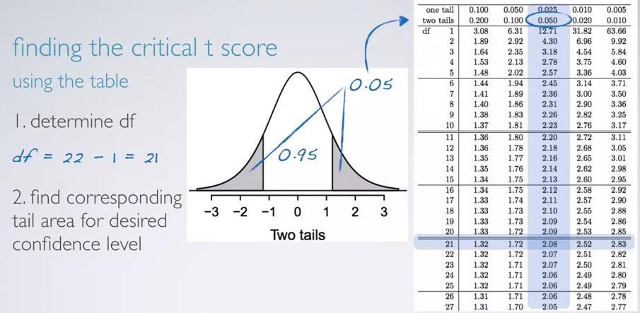
We already have our df, and we can point that horizontally if we use a table and mark df 21. Next, it depends on our question. Since confidence interval is always concern about two-sided, we can search the corresponding with two-tails equal the rest area, 5% if we're looking at 95% confidence level. Then we will find 2.08 as our $t_\mathbf{df}$.That's from table. now calculating with R,
%R qt(0.025, df=21)
This is similar to what we did in qnorm function, and remember to always take positive values.
Screenshot taken from Coursera 09:57
%%R
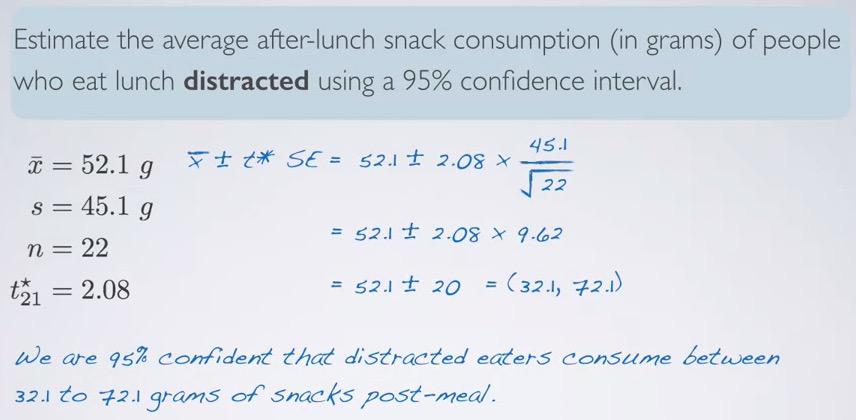
n = 22
mu = 52.1
s=45.1
CL = 0.95
z = round(qt ((1-CL)/2,lower.tail=F,df=n-1),digits=2)
SE = s/sqrt(n)
ME = z*SE
c(mu-ME,mu+ME)
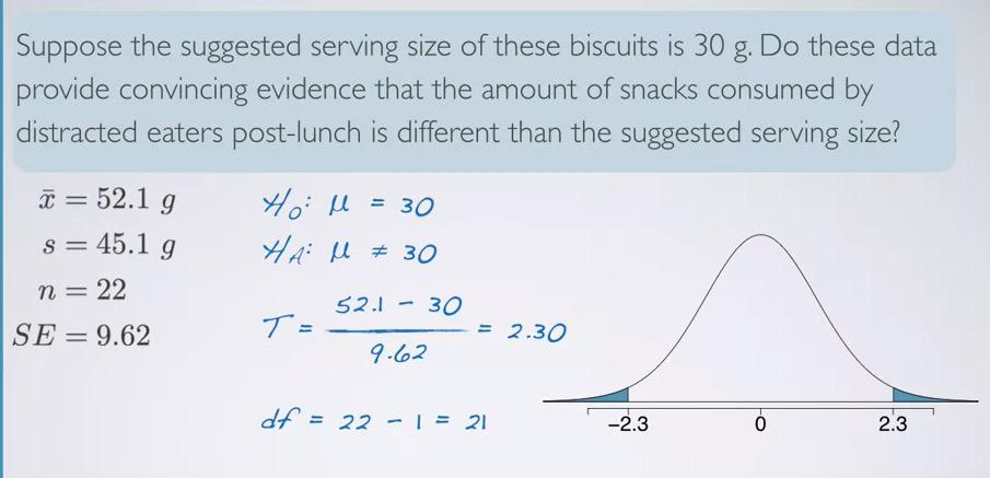
For hypothesis testing,recall that null hypothesis is the skeptic, we're testing whether our data provide strong evidence for existing hypothesis. In this problem, the existing one is suggested serving size 30, which will be our null value.
Screenshot taken from Coursera 15:49
%%R

xbar = 52.1
mu = 30
sd = 45.1
n = 22
SE = round(sd/sqrt(n),digits=2)
t_star = round((xbar-mu)/SE,digits=2)

pt(t_star, df=n-1, lower.tail=xbar < mu) * 2
%%R

xbar = 52.1
mu = 30
sd = 45.1
n = 18
SE = round(sd/sqrt(n),digits=2)
t_star = 0.5
# round((xbar-mu)/SE,digits=2)

pt(t_star, df=n-1, lower.tail=T)
Is the HT agrees with CI in this case? 30 is not in the (32.10007 72.09993) interval, so yes, it agrees.
Conditions are also must be checked:
- Independent - random assignment. You see that this is an experiment, and they're doing random assignment to treatment and control groups
- Independent - less than 10% distracted eaters. It's also true, the sample size is 30.
- Skewness. This is unknown to us. However we can infer the shape based on the data that we have. We know that $\bar{x}$ = 52.1 and $s$ = 45.1. There's no way grams are negative, so it always be positive. standard deviation is huge, so we can only observe a little above one standard deviation in the left, and largely towards the right (intuitively, fewer people will have larger snake intake).
Inference for comparing two small sample means
Now we will compare two groups with small size, using our examples earlier.
Screenshot taken from Coursera 02:20
Screenshot taken from Coursera 03:42
So the formula is still the same. You have same calculations when you comparing two large sample means on HT and CI, you have same calculations when you calculate HT and CI for one sample means using t-score, but the difference is the option on how to pick degree of freedom. This is simply going to get the minimum of 2 df samples. In reality, is not that easy however, there's more complex calculations(too complicated by hand), but it still serve as a good estimate.

Screenshot taken from Coursera 07:30
Keep in mind that our standard error is get by not incorporating standard deviation, but actually the variance. In standard error for one mean you do $\frac{s}{\sqrt{n}}$, but it's actually $\sqrt{\frac{v}{n}}$, where standard deviation is just the squared root of variance, so we exclude that from sqrt.Now for calculating SE for two sample means, we put it back as a variance.Since t-score is similar with what we get when we calculate one mean earlier, it's still somewhere between 0.002-0.005 for the p-value.
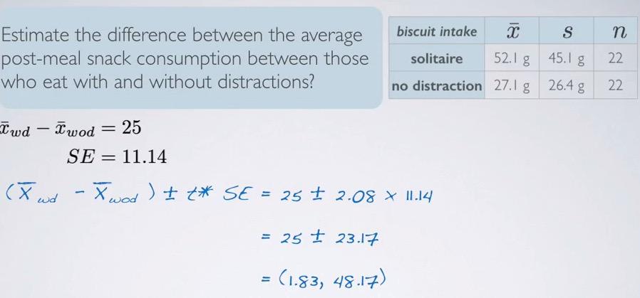
So we can conclude this data is provide convincing evidence that there is a different of snacks intake post lunch, between those eating with distractions and those that are eating without distractions.
Screenshot taken from Coursera 08:39
So we can say that we are 95% confident those with eating distractions consume between 1.83 to 48.17 grams more snack to those without distractions, on average.
Is HT agrees with CI in this problem? Yes. Since the null value is zero, and zero is not in the interval, HT agrees with CI.
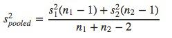
Pool standard deviations, is when you have very rare conditions where the standard deviations of the population being compared is really similar.
Screenshot taken from Coursera 08:39
Comparing more than two means
Up until now we only make an inference of one mean, inference of two means, but never more than that. This section want to tell how to make a comparison, inference-based for more than two means.
Screenshot taken from Coursera 00:56
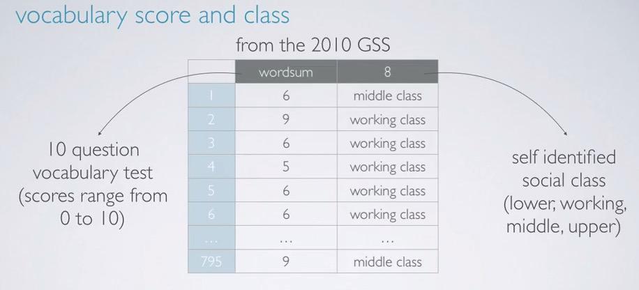
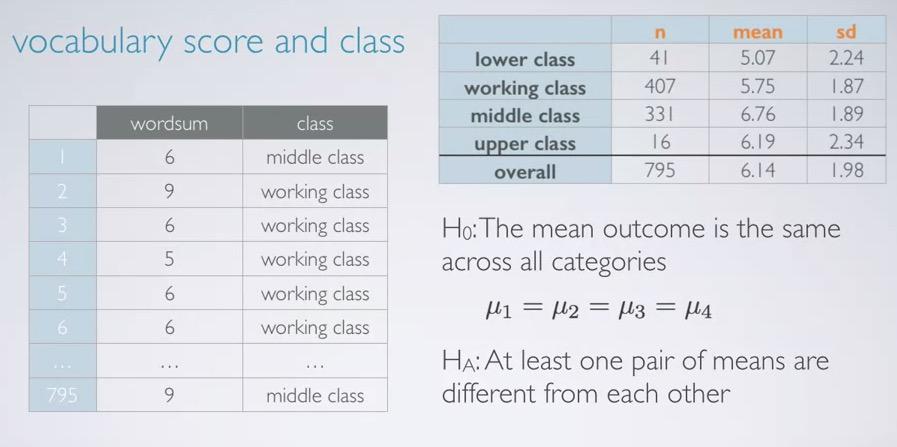
We will use an example of 2010 GSS data where we compare the vocabulary test consist of numerical discrete to self-answered social class, category.The distribution of the samples is unimodal, and slightly left-skewed.For doing the analysis you can first plot a histogram for all the scores, you can do a bar plot to see the frequency of each social class, you can do side-by-side boxplot for category-numerical, and lastly, calculate summary statistics for each of the social class.
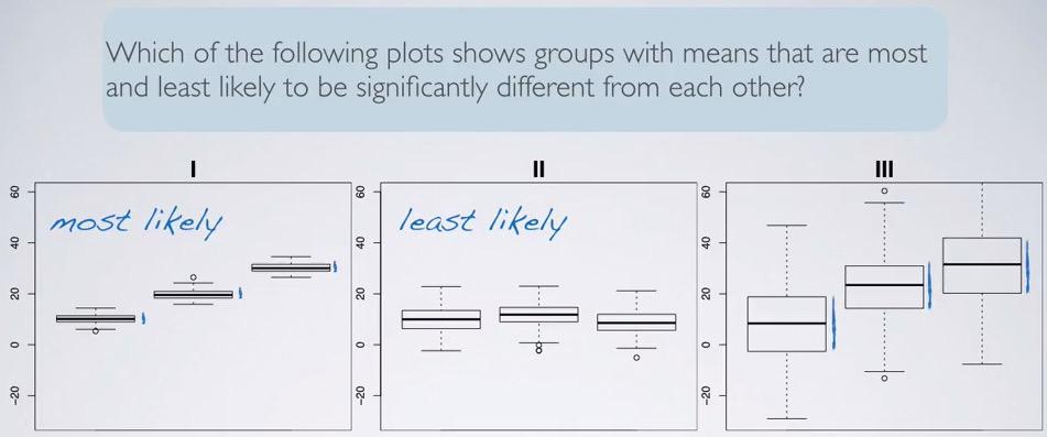
Screenshot taken from Coursera 04:42
If we're looking at the three boxplots here, 1 is most likely significant. Why? Because the IQR is small, and each of them not capturing other means with their IQR. so the means is significantly different in 1. The less likely is plot 2. It's almost no different with their means, and all of them can capture the means of others.
So in this context, we have a questions, "Is there a difference of vocabulary scores between social (self reported) classes?
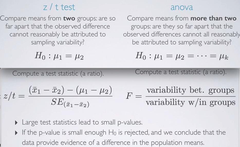
- To compare means with two groups, we use t or z statistics.
- To compare means for more than two groups, we use analysis of variance (ANOVA) and use new statistics, F.
Summary
- small sample size (< 30) follow t-distribution more than normal distribution, to accommodate skewness/variability of the data compare to normal distribution.
- t-distribution is different than normal distribution, t-distribution has single parameter, df, and normal distribution has two parameter, means and standard deviation. Heavy tail in t-distribution will accommodate the skewness/variability resulting in small sample size.
- The calculation for confidence interval and hypothesis testing is still the same, except the calculation for t_score. For one sample mean, you calculate still the same. For comparing two means, you calculate standard error like two independence means, and degree of freedom is the minimum of each sample size minus 1.
- t-critical score will be get by using qt function in R, you can see that at 95% confidence level, t_score is higher than z_score, as you recall tht t_score has higher variability.
ANOVA
If earlier we use hypothesis test for more than two means, we set the hypothesis test.As always, null hypothesis is the skeptic one. There is no difference going on of means across groups
$$ \mu_\mathbf{1} = \mu_\mathbf{2} = ... = \mu_\mathbf{k}$$
Where $\mu_\mathbf{i}$ mean for outcome in category i,
k = number of groups
The alternative hypothesis is however at least one pair of them is different from the others. We don't how many of them are different, we don't know which of them is different, all we know is we're only have the probability of at least one of them is different. Recall that probability:
P(at least 1 | 5) = 1 - P(none)**5
Screenshot taken from Coursera 08:42
So, once again if z/t test calculating the difference whether sampling variability or not, in anova we test all of them produce p-value of sampling variability.
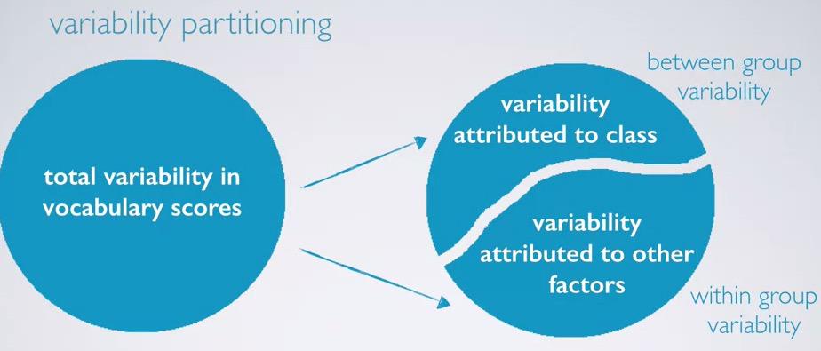
If we calculate the difference between two means for each of their respective groups, in anova we calculate the variability across groups, and within groups. Recall that HT is rejected if p-value smallls(contributed by large test statistics) and conclude evidence of difference in the data.
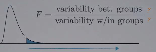
Screenshot taken from Coursera 09:38
F-distribution is right skewed, and we shaded the positive area. We're going to reject small p-values, which are contributed by large F statistics. In order to do that, mathematically, variability between groups must be larger than variability within groups.
So we can use anova when we want to detect a different of point estimate across groups. Perhaps students' final exam can be contributed by many factor, how many hours per week,quiz,midterm,project,assignment and so on and so forth. This have many category, and we want to ask which of the groups has variability that happen by other reasons.
Screenshot taken from Coursera 02:04
Recall in this data, our vocabulary score data with the social (self reported class). Also we are given summary statistics for each of the class. Null hypothesis is being skeptic one that there is no difference, and alternative at least one of them is different.The explanatory is social class, and the response is vocabulary score. This study is first divide the the data into categorical (social class), and then analyze the vocabulary score(numerical). We want to see whether the social class affect the score, and summary statistics show us that first separate by class and summary statistics taken from vocabulary score.
Screenshot taken from Coursera 03:17
After that we analyze the variability of explanatory variable. What we do is actually observe if the vocabulary score vary because of class or other factors. So after we separate by class, is the variability within groups, other than class, is larger than the variability by class? If indeed larger, then F statistics will be smaller. On the other hand, if variability between groups is larger than within group, then it will result into large F statistics.So F statistics will be large if variability of explanatory variables is the largest among other categories all combine into one.
Screenshot taken from Coursera 03:40
Sum Sq
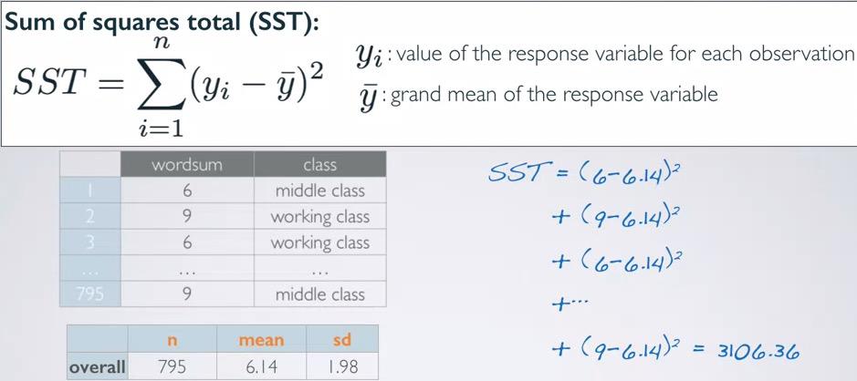
Sum of Squared(SST)
Screenshot taken from Coursera 07:29
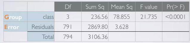
The value total (3106.36) is often called sum of squares total (SST). It's calculated by SST of response variables before explanatory separation (vocabulary scores in total). It's similar to variance, but it's not scaled by the sample size.Remember that variance is calculated by SST divided by sample size.
Recall that finally what we're trying to find is hypothesis testing based on the p-value. And p-value is get by calculating F statistics, which composed to the ratio between variability across groups to variability within groups.
SST not benefit if we only calculate this. We're going to step through all the value in ANOVA table.
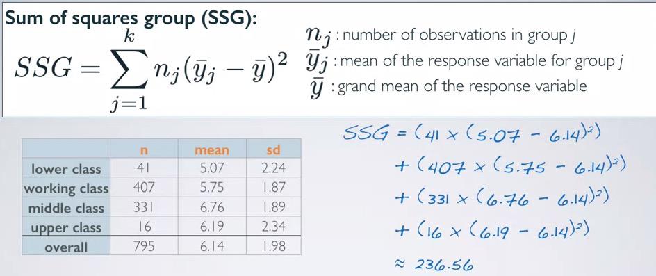
Sum of Squared Groups(SSG)
Screenshot taken from Coursera 10:14
The value of 236.56 measures the variability between groups(explanatory variable). We're going to take mean of each of the group and its sample size, and create a deviation of group mean from overall mean, weighted by sample size.
SSG is similar question from SST, except that it weighted by sample size. Recall that SST measures the variability of total response variables, SSG measures the variability of mean of each explanatory groups. This will give us 236.56.The ratio is important though(not magnitude, don't pay attention to the large value, but how it ratio to the SST), and we can see that sample size will also comes into play (larger data could weight more to the grand mean).
Sum of Squares Error (SSE)
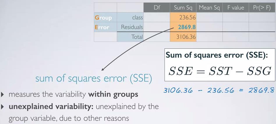
Screenshot taken from Coursera 12:23
Lastly, SSE is just the complements of the SSE and SST. What are the variability of the data other than explanatory variables. In other words, variability within groups. This could be other reason. And by looking at the ratio, it's large enough compared to SST. Which makes sense, as background in education, IQ, etc could be be stronger factor compared to social class for determining variability of vocabulary score.
Mean Sq
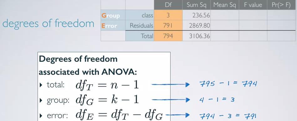
So after we get SSq, we also looking for a way to convert the total variability into average variability. And that will require scaling by a measure that incorporates sample size and number of groups, hence degree of freedom.
Screenshot taken from Coursera 14:02
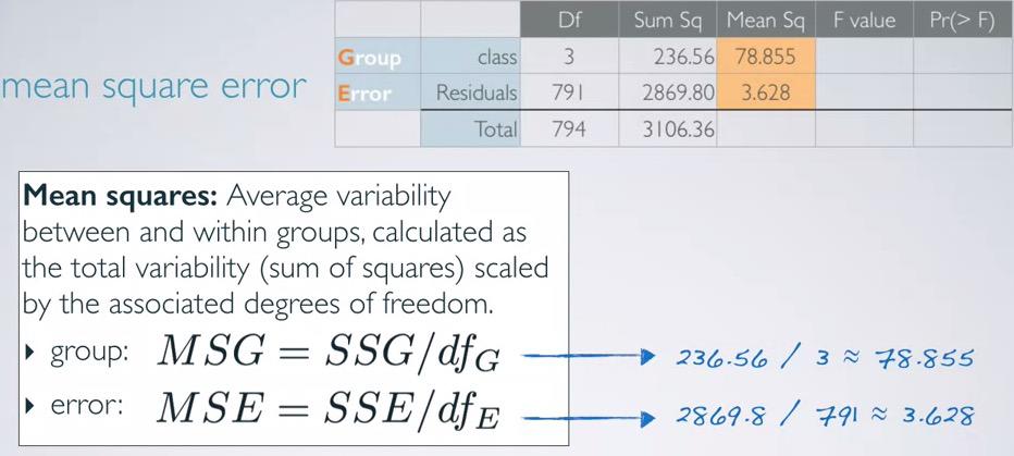
The degree of freedom then will be easy to calculate. We already know sample size, we already know the number of groups, just plug in to the table. The mean squared error will be filled by sum of squares, scaled by degree of freedom.
Screenshot taken from Coursera 15:19
IMPORTANT. Before, we calculate the residuals for both df and SSq by calculating the complements of total and class. For MeanSq, we're calculating it by averaging its df and SSq.
F statistics
Screenshot taken from Coursera 16:13
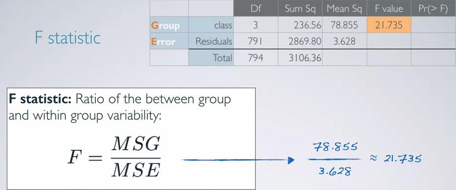
F value then converge into one row, incorporates MSG and MSE. Again, we know that F statistics gives us the ratio of variability between groups compared to variability within groups.
Screenshot taken from Coursera 17:26
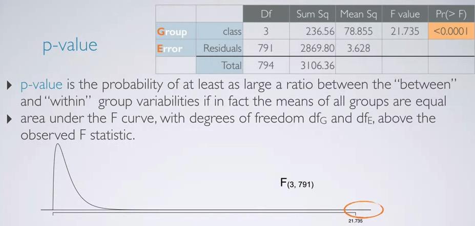
Recall that p-value is the probability of at least as extreme of an observed outcome given the null hypothesis is true. So p-value for f statitics is probability observing the ratio of variability between groups and variability within groups at least as extreme given mean of all groups are equal.
The area that p-value observed is with dfg and dfe parameters, observe at lease 21.735. This will gives us very small p-value in the example.Notes that the distribution is right skewed, and so even we observe the different, we calculates one tail instead of two tail.Mathematically, Sum of a squared numbers will gives positive number, and degree of freedom is number of sample size, so that also positive number. Both can't be negative,The distribution can only be tailed to extreme positive, thus we're only observing the positive side.
Using R, we can specify F-value,dfg, and dfe, and we also shade the positive area, which false in the ower tail
%%R

f_value = 21.735
dfg = 3
dfe = 791

pf(f_value,dfg,dfe,lower.tail=F)
Using applet you can go to http://bitly.com/dist_calc
k = 5
K = k*(k-1)/2

0.05/K
If p-value < $\alpha$, the data provide convincing evidence that at least one pair of population are different from each other (we can't tell which one).In this case we reject the null hypothesis.
If p-value > $\alpha$, the data doesn't provide convincing evidence that one pair of population means are different from each other, the observed difference is due to sampling variability(or by chance).In this case we fail to reject null hypothesis.
Since p-value is really small in this problem, we reject the null hypothesis, and conclude that the data is provide convincing evidence that at least one pair of population means are different from each other.
Conditions for Anova
The conditions area:
-
Independence:
- within groups : sampled observations must be independent
- between groups : groups are indpendent of each other (non-paired)
- Approximate normalty. Within each group, the distribution must be nearly normal.
- Equal variance. The variability of all groups are roughly equal.
We're going to discuss these parameters one by one.
Independence
First, you want to do random sampling/assignment depending on whether you use observational or experiment. This will ensure the independence of the data. Same as you did since CLT. You also want to ensure that each of the group have sample size less than 10% of population.
Be curious about the data, you must know that each of the group is independent of one another. This sometimes difficult to do when you have data gathered by someone else, or you get other sources in the internet. One way to do so is take repeated measures of anova.
Approximately normal
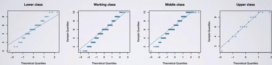
Screenshot taken from Coursera 03:34
Next, you want to ensure that the distribution within each group is approximately normal. This to ensure that groups have same variability. It's more important when the sample size is small. You can see that lower class and upper class have small sample size. The jumps occured because the score is a whole number(no decimal).
Constant Variance
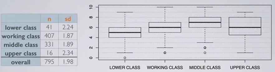
Screenshot taken from Coursera 04:47
The variability, variance is equal for each of the group. This especially important when sample size is differ. You can observe variability based on variance(boxplot), sample size and standard deviation. You can see that upper class have wider variance, and you see that it has small sample size.
Multiple Comparisons
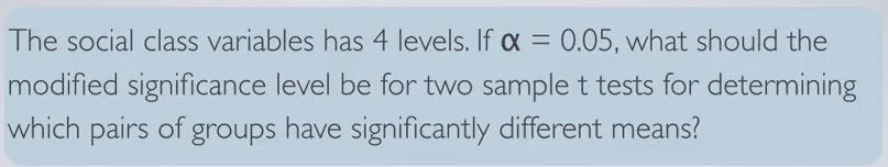
If before we don't know which means are different, this section will get us multiple comparison to finally find the mean. This may pile up type 1 error, so we have to find a way to keep getting it constant.
One way to do this is to perform two sample t tests for each of possible pair in groups. We talked about how it will increase type 1 error rate, and the way to solve this is by using modified significane level.Think about it, if only fixed significance level of 5% of each pair, the number of comparisons would yield less and less than 5%.
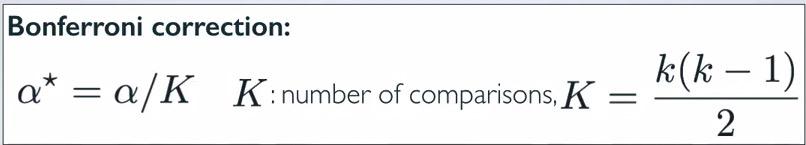
These comparison of each of possible pair of groups is called multiple comparisons. You usually do multiple comparisons when you know that your F-test has significant result. Bonferroni correction will be used, stating that more stringent significance level must be use in this case. the significance level then will be depend on number of multiple comparisons that you have.
Screenshot taken from Coursera 02:35
Screenshot taken from Coursera 03:52
Recall that k= number of groups,
$$ K = \frac{4x3}{2} = 6 \\ a* = 0.05 / 6 \approx 0.0083 $$
%%R

k = 5
SL = 0.05

SL/((k*(k-1))/2)
So as you can see have much smaller significance level, resulting in more stringent threshold to reject null hypothesis.
Pairwise Comparisons
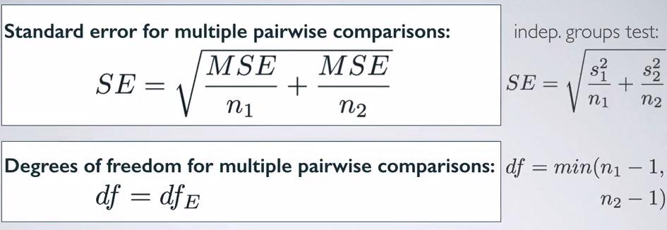
So after you're doing multiple comparisons after ANOVA, you want to recalculate standard error and degree of freedom. This standard error and degree of freedom must be the same regardless of standard deviation or sample size for each of the test. It has to be consistent. Then compare the p-value of each test to the modified significance level.
Screenshot taken from Coursera 05:54
So again, we see similar calculation for calculating standard error and degree of freedom in t-distribution independent means. But now instead of using variance of the sample, we're using MSE (mean squared error). So the standard error will be square root of sum of MSE divided by each of the sample size. And instead of finding minimum of sample size for degree of freedom, we're using degree of freedom for residuals.Let's test this based on the same example earlier.
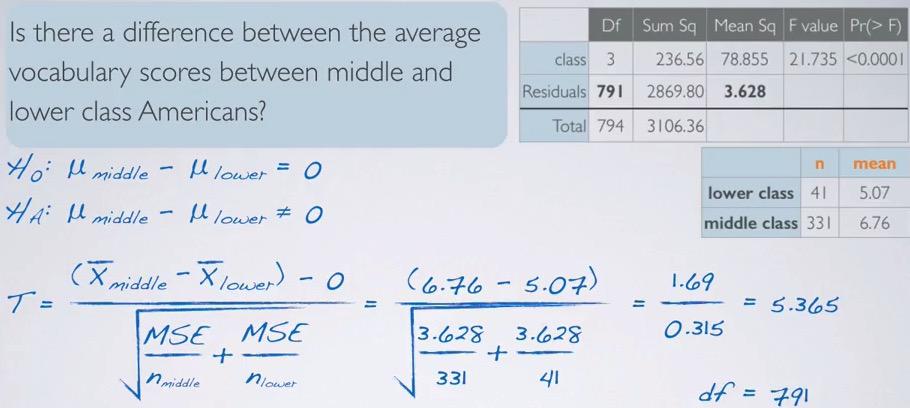
Screenshot taken from Coursera 08:19
Given the problem and tables provided, we're going to calculate the p-value. So we're going to calculate t-statistic for hypothesis testing of whether middle and lower class is difference. The null value as usual will be 0, and the alternative is middle and lower class are different. Put in t statistics, gives us calculate the of difference of mean divided by standard error that we learned recently, resulting in 5.365.Remember that degree of freedom also use degree of fredom in residuals, so we're using 791.
Screenshot taken from Coursera 10:22
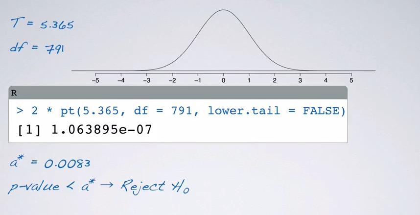
So why this looks like a normal distribution instead of right skewed distribution? Because we already convert it into standardizing normal distribution, and the null value is zero, so the distribution is centered around zero. The degree of freedom is also very high it's approximate normal distribution. You see that t statistic is z-score, and z-score with more than 5 standard deviation will result in very small p-value, using R,
%%R
T = 5.365
df = 791

2 * pt(T,df=df,lower.tail=F)
So you see that even significance level has beeen modified, to adequate 5% level, p-value is still smaller. Therefore we reject the null hypothesis, and the data provide convincing evidence that average of vocabulary scores between self-reported middle and lower class Americans are different.
Summary
ANOVA is statiscal tools that lets you analyze many groups at once. Is it due to chance variability of particular groups compared to variability of others? Different from usual HT, in ANOVA you set null hypothesis to be equal means across groups. But in alternative, you want to observe at least one group is different. Two probability, either all equal, or at least one different.
Conditions for ANOVA is at independence for between groups and within groups. The distribution of each group is nearly normal, and you variability across groups also nearly normal. Use graphical tools like boxplot and summary statistics to make intuition about the data. F-statistic will be get by calculating MSG with MSE, the means will calculated by dividing the sum of squares with its corresponding degree of freedom.This is right skewed distribution, you won't be have negative number, which always yield positive number. There's fore we always use one sided p-value.
Recall that we have 5% type 1 error rate for one hypothesis test. Doing multiple test will pile up the error, so fix number of 5% is not enough. We have to always push down the error rate, and by doing that incorporate with K-value.It's possible that when you reject the null hypothesis(statiscally significant) in ANOVA, but end up not finding it when you test it between groups. Remember that ANOVA is about at least one is different. And you may only one group that is different, but not for the rest of the groups.