So far we've been looking into the problem where we have single categorical/numerical, relationship between categorical-numerical or categorical-categorical. In this blog, we're going to discuss about two numerical variables. We have a correlation test, want to test the strengthness relationship of both numerical variables, inference, and introduction to linear regression.For those that familliar with machine learning, this blog will make additional flavour from statistics.Why is it call linear regression? Because it's all about regress towards the line.

Correlation

Screenshot taken from Coursera 01:00

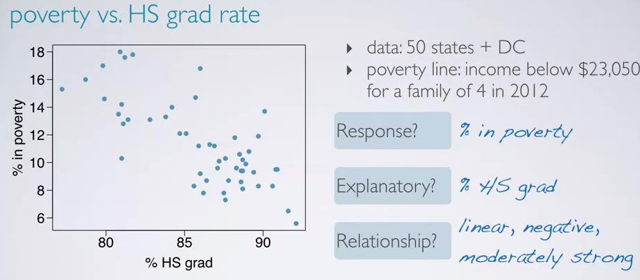
The picture above is about the rate between poverty and high school graduate in the US. First we have poverty rate, as response, and we want to see whether it's affected by HS graduate, the explanatory. When looking into two numerical variable, we often observe the linearity, the direction, and whether both have strong correlation.Correlation here means linear association between two numerical variables. Non-linear will be just called association.

Correlation is all about linearity, and often called linear association, and it's denoted by R.The explanatory acts as a independent variable(predictor), and the response variable is the dependent variable.We can see the linearity, by looking at the foremention 3 categories:

Screenshot taken from Coursera 02:00

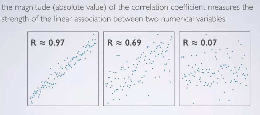
The higher the correlation(absolute value), represent the stronger relationship, linear between both variables.

Screenshot taken from Coursera 02:28

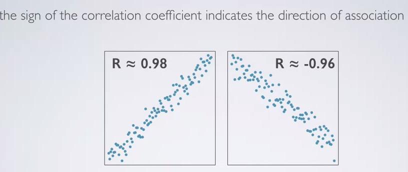
The direction of the linear decide sign value of R.

Screenshot taken from Coursera 03:09

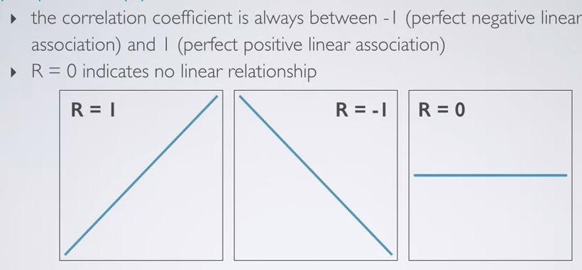
The linear will always between -1 and 1. It will fall perfectly in a line. Whereas 0, as you can see x increases, but nothing's to do with y.

Screenshot taken from Coursera 04:30

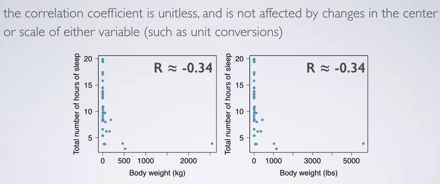
R is unitless, meaning no matter how you change the unit, or scale, it will always retain its value. Here we have R close to zero, and you can see based on the previous example, it almost show no correlation.

Screenshot taken from Coursera 05:11

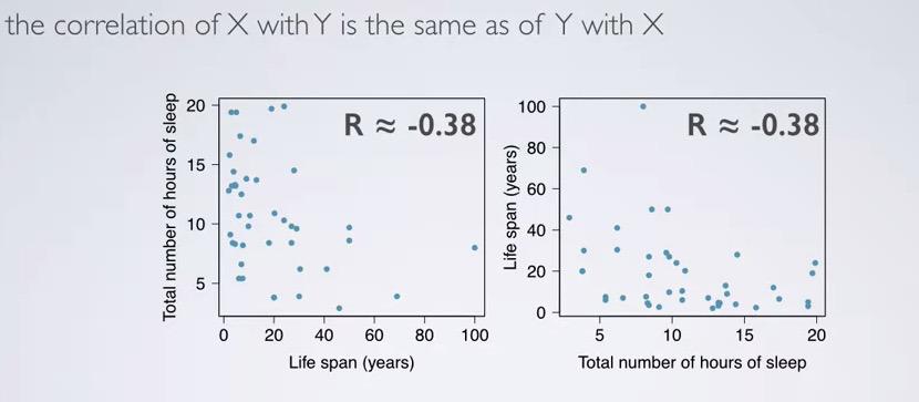
Even if you flip both axes, R will still be the same.

Screenshot taken from Coursera 06:15

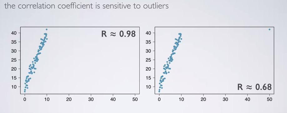
When you move even 1 point to corner outliers, R will vary significantly. correlation coefficient is sensitive to outlier.

Screenshot taken from Coursera 08:20

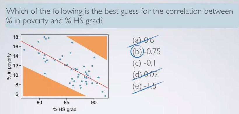
Take a look at the example. correlation coefficient is always between -1 and 1. So you can eliminate e. Its direction is negative, so it only betwen b and c. All that's left is strong/weak correlation. Try to imagine the negative space (shaded by orange color). This will help us better intuition. R with 0.1 will almost not give us negative space.

Residuals

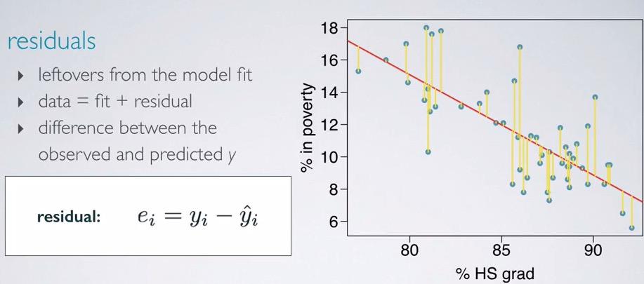
Screenshot taken from Coursera 00:44

Residual is the distance between the actual output of y-axis and your hypothesis. This will serve as a basis of predicting the output, in this case poverty. So given grad rate, we want to predict rate in poverty. What we want to do is minimizing the residual overall.

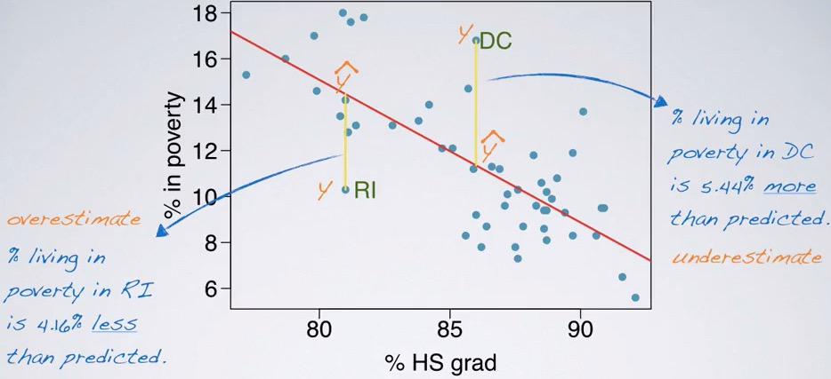
Screenshot taken from Coursera 01:44

It will overestimate if the predicted is beyond the actual output, and underestimate if the predicted below the actual output.

Least Squares Line

In this section we want to talk about how we minimize the line in linear regression, by taking least squares (cost function).There's another option where we talk about the distance error as the absolute value, but as we talk before, we want to give higher magnitude to those with longer distance. So we squares all distance, this also give advantage as it's easier to calculate and more common.

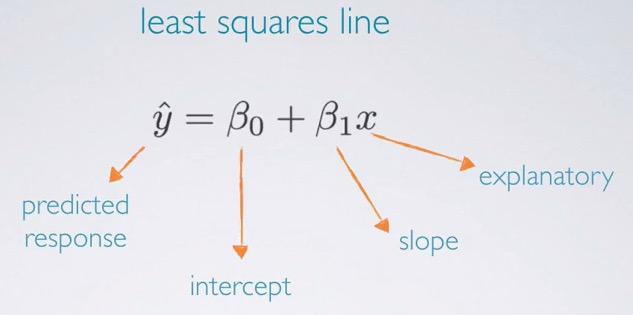
Screenshot taken from Coursera 01:24

So this would be familliar to those with machine learning experience. We have $\hat{y}$, as our hypothesis, the predicted output. We have intercept, as a bias unit. We have the weight parameter, a slope that can then multiplied by explanatory variable. We have seen this formula, when we're calculating gradient in high school. Recall that y = mx. With m the slope, and we have additional bias unit.

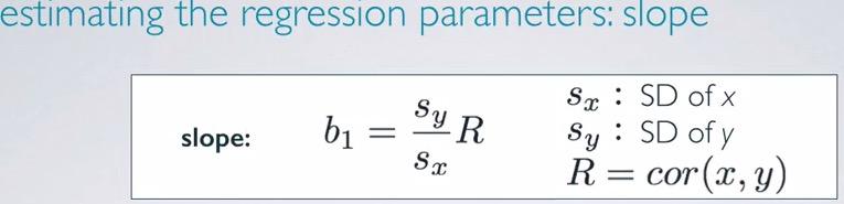
Screenshot taken from Coursera 02:44

Here we have b1, as our slope point estimate (b0 will be represented as intercept point estimate). And the calculation of b1 is just swapping from previous formula.So the slope is standard deviation of response variable, times correlation coeffecient for response-explanatory, divided by standard deviaton of the explanatory variable.

$$ b1 = \frac{s_y}{s_x}R$$

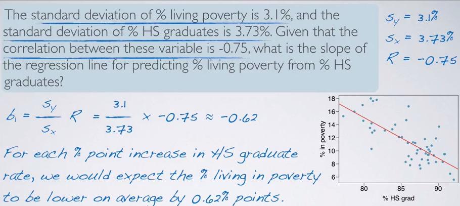
Screenshot taken from Coursera 06:08

Here we simply have all the parameter, and can calculate the slope. Standard deviation is always positive for both response and explanatory (as you recall, it derrive from squared difference). So the sign of the slope is always depends on the sign of the correlation. If you see the image, you can see that it has negative direction.

Since we're talking about the percentage rate, 0.62 is the percentage, so we can say that percentage living in porverty is lower(negative sign!) on average by 0.62%. Mind that since this is observational study, pay attention that we're trying to make a correlation and not causal statements. So 'would expect' is the chosen phrase instead of 'will'. And explanatory variable is the one unit meassurement to the predicted response variable. So we have one unit (percentage), so we say as one percent of HS graduate increase, we would expect poverty to be lower on average by 0.62 %. Pay attention to the units of response and explanatory, as both can be different.

Screenshot taken from Coursera 07:11

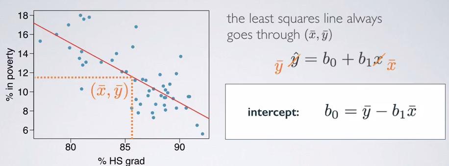
We can replace the formula with $\bar{y}$, which denotes the average of response variables, and $\bar{x}$, which denotes the average of explanatory variable.The intercept will then simply swapping the parameters.You see that in linear regression, it expected that the line is go through the center of the data. Which means, the line is all of the average of data points.

Screenshot taken from Coursera 09:28

linear regression is always about the intercept and the slope. Explaining intercept alone is less meaningful. Recall the formula as:

$$\hat{y} = \beta0 + \beta1\hat{x}$$

So when the explanatory variable is zero then,

$$64.68 = \beta0 \\ \beta0 = -64.68 $$

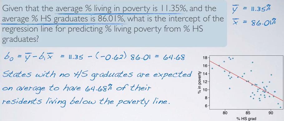
Based on the formula, simplifying to just the intercept, as the picture stated, "States with no HS graduates(assumed zero explanatory for the sake of statement), are expected to have 64.68% of their residents living below the poverty line(response).

Screenshot taken from Coursera 10:38

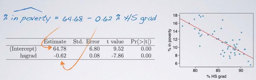
By doing computation software, the table shows the intercept and slope in the estimate column, while the rest of the table will be explained later.

So in intercept, explaining only that will provide no useful information. you only setting the x = zero, which will intercept at the y-axis. And intercept only benefit as provide base y-axis(height of the line). While slope, explaning the correlation of x/y axis. As x increase(each unit), what happen to the y-axis(higher/lower?) on average.

So least squares line always passes through point average of explanatory and response variable. Using this idea, we can calculate the intercept value as:

$$ b_0 = \bar{y} - b_1\bar{x}$$

there are different interpretation depending on whether you use numerical/categorical explanatory variable.To interpret intercept when x is numerical " When x = 0, we would expect y to be equal on average to {intercept}". When x is categorical, "We expect the value average of response variable for {reference level} of the {explanatory variable} is {intercept value}".

and the slope like before calculated as:

$$ b_1 = \frac{s_y}{s_x}R $$

To interpret slope, If x is numerical " For each unit increase x, it's expected an increase/decrease by {slope units} for y in average". When x is categorical however, we say, "The value of response variable is predicted to have {slope units} higher/lower between reference level and the other value of explanatory variable. Increase/decrease is depend by sign of the slope.

So indicator is the binary explanatory variables. And based on this fact, we can interpret intercept(with level 0) and slope(with level 1).

Suppose we're given this example,"The model below predicts GPA based on an indicator variable (0: not premed, 1: premed). Interpret the intercept and slope estimates in context of the data."

gpaˆ=3.57−0.01×premed

For the intercept, "When premed equals zero, we would expect gpa in average to be 3.57". For the slope, "For each increase of 1 premed, we would expect the gpa on average to be lower on average by 0.01 unit"

xbar = 70
xs = 2

ybar = 140
ys = 25

R = 0.6

slope = (ys/xs)*R
intercept = ybar - slope*xbar

c(intercept,slope)

[1] -385.0    7.5

xp = 72
yp = 115

predicted =(intercept + slope*xp)
yp - predicted

[1] -40

Prediction & Extrapolation

Recall that in the prediction, we're going to map x into the line, and infer y based on the point projected on the linear regression. In other words, which y-value that correspond to given x-value that construct point in the linear regression.

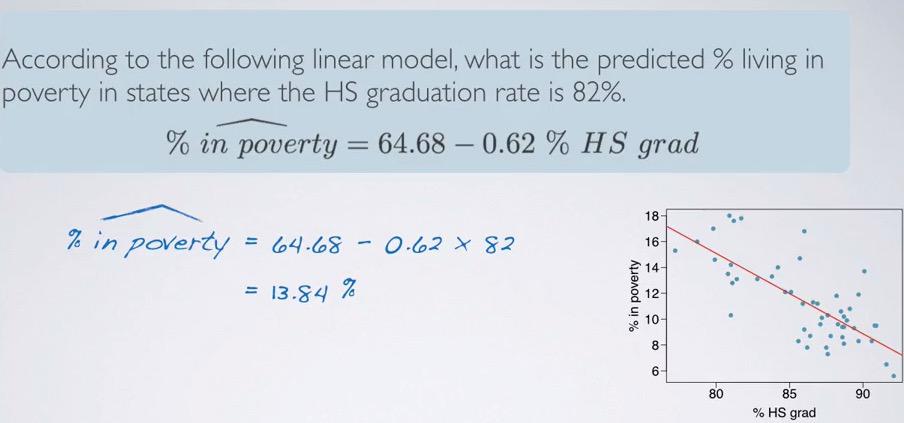
Screenshot taken from Coursera 10:38

Using intercept and slope from previous example, we can simply plug the explanatory, 82 to the resulting formula. What we get is 13.84. So based we can say on states, given that the state have 82% HS graduation rate, we predict that 13.84% on average in the poverty line. But beware of some extrapolation.

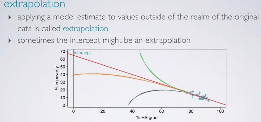
Screenshot taken from Coursera 02:49

Extrapolation would means that we want to infer something outside realm of the data. The data that we have are the explanatory in range from 70-95(more or less). But far more outside the realm, we don't know if the intercept consistent with linearity, or maybe in exponential(logistic) manner. Take a look at the red line, intercept with the red line would be wrong. And any exponential line would interpret wrong result outside the realm.

So if the problem will need you to predict the poverty rate at 20% HS graduate, you can't do that. The resulting estimate will yield unreliable output.

So we can predict for any given value in the explanatory variable, x*, the response variable will be:

$$ \hat{y} = b0 + b1x^*$$

Always remember to not extrapolate response variable beyond the realm of data.

REFERENCES:

Dr. Mine Çetinkaya-Rundel, Cousera