Probability

The probability is a branch from statistics. We can rely on probabillity to predict what kind of value comes out from the population.Probability defines in mathematical formula as follow:

$$0 \leq P(A) \leq 1$$

For probability there are two popular definitions:

• frequentist interpretation. It is the traditional method which explain the probability that observe a random process of infinite number of times, and get proportion of each of the outcomes out of all outcomes.

• bayesian interpretation. It is the probability of two point of view observe an event. This maybe perhaps two different kind of view, a prior, which will be sometimes included in statistical inference, is a view before it's observe an event. And posterior, is the probability after observe an event. Bayesian method has been largely used in technology and methods for the last twenty years.

Random Process

Random Process is the process in which we know all possible outcomes, but don't which outcomes that will get out. You know two sides of coin, but don't know which side will come out in coin toss. Or a number that comes out in a dice, or a music comes out in your playlist. It's often useful if we random first our possible outcomes.

Law of large numbers

Law of large numbers states that if you observe a probability of an event, approach infinite number of times, the probability will converges to probability of an outcome. Say if you roll a dice and number 5 comes out, the probability of 6 will be 1. If you roll for the second time and 4 comes out, the probability comes out 6 will be 0.5. And if you roll thousands and thousands more, it will converge to the actual outcome, 1/6.

The law stated that when sample size is few, the probability between events may because due to chance. But if the size is large, say over thousands, the probability won't likely happend due to chance. It's maybe usual to find 7 heads in 10 coin toss for fair coin, but unusual for 700 heads in 1000 toss.

Law of averages (gambler's fallacy)

Law of averages is on the other hand is oppose law of large numbers. Law of averages incorporates the observation that happen in the past. The probability of coin toss for tenth time is not suppose to remember the outcome for all previous nine toss. If thousands of coin toss but head still comes out, that it maybe not a fair coin. But it still doesn't remember for what occurs in the past. If observe, then the probability is times the previous one, is called law of averages.

disjoint (mutually exclusive)

disjoint events can't happen in the same time.

Example : A coin toss can't come out with head and tail.

The formula then

$$P(A and B) = 0$$

non-disjoint events on the hand, can happen in the same time.

Example: A worker is in the office for Monday and Tuesday.

$$P(A and B) \neq 0$$

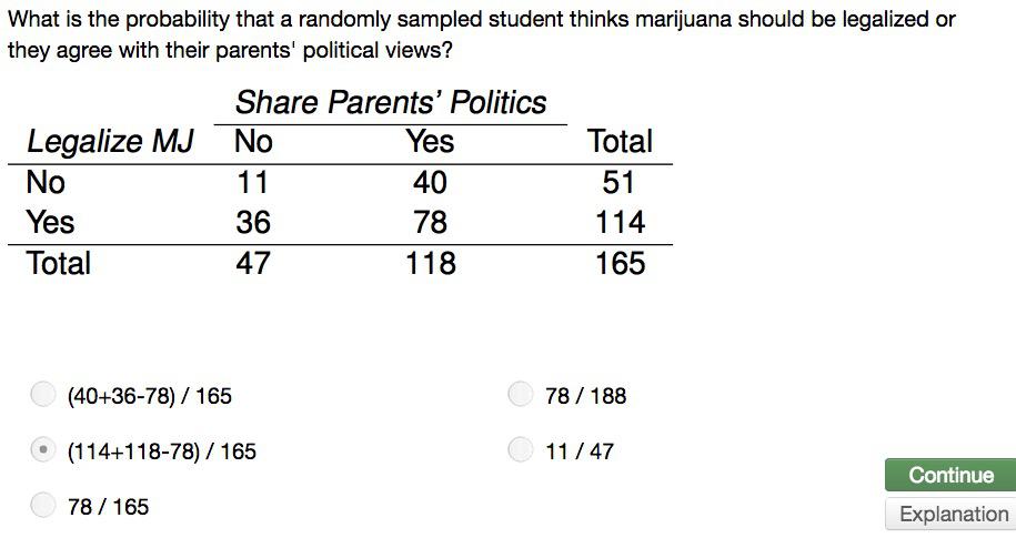
union of disjoint events is the probability of two or more disjoint events. For example,getting Jack and Three from well-shuffled deck of cards.For disjoint events A and B, the probability is simply sum of two events.

$$P(A or B) = P(A) + P(B) $$

union of non-disjoints events, on the other hand is a little bit tricky, we want to subtract the probability of overlapping events, to avoid double counting.For non-disjoint events A and B,

$$P(AorB) = P(A) + P(B) - P(AandB)$$

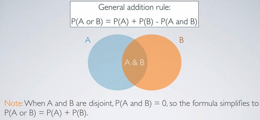
Screenshot taken from Coursera video, 05:11

Overall disjoint events only need to remember about one thing. In this general formula, the overlapping events will be zero, and thus will get ignored.

Screenshot taken from Coursera video, 05:11

Sample Space

Sample space is collection of all possible outcomes of a trial. If for example if the parents has two childs and predicts the outcome, we can make a trial to infer all possible outcomes.

S = {MM, FF, FM, MF}

Probability distributions

Based on sample space that we gain earlier, we can make probability distributions which listed all possible outcomes and its respected probability. For example and rules:

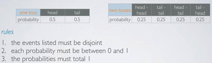
Screenshot taken from Coursera video, 07:07

Complementary Events

The complementary events is the sum of all the rest of the probability other than observed event. The complementary events of head occurs in one coin toss, is the probability of tail comes out. Two head-head event, the complementary events is the tail-tail, head-ail, and tail-head.

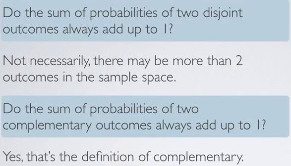
Screenshot taken from Coursera video, 09:15

So an event and its complementary events is always two disjoint events, and add up to 1. But the two disjoint event can't always add up to 1, since there might be other disjoint events. Republican and Democrat population can't be add up to 1, since there might be Other or Independent population.

Independence

The two processes are known independent, if the outcome of the first one provide useless information to the second one. Here's the example:

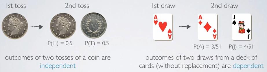
Screenshot taken from Coursera video, 01:17

Coin Toss is always an independent outcomes. The draw of deck cards will become dependant, if the previous draw doesn't return back to the deck. In the right you see that Because Ace Red drawn from the first step, the probability of Ace Red in the second draw, will get affected, also in Jack Spades. 51 is number of cards after we pick the first draw and not returning it back.

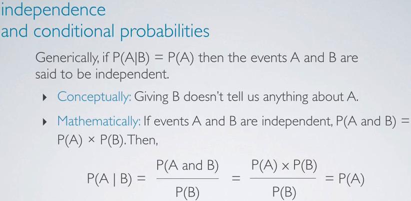
The general formula then become, for checking an independence:

If P(A|B) = P(A), then A and B are independent.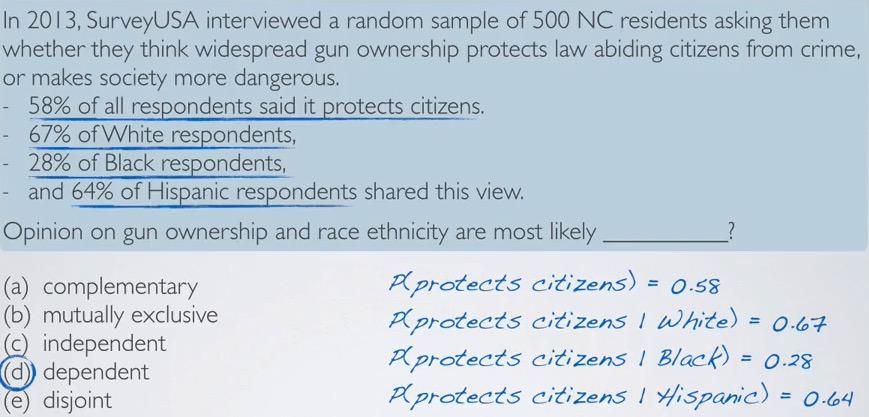

Let's take an example:

Screenshot taken from Coursera video, 01:17

A : Race Ethnicity
B : 'protects citizens'

Since the probability of P(A|B) $\neg$ P(A), and it varies greatly for each of the A, then the two event is dependant. The probability will be the same regardless of the A, if the two events are independent.

In the observation of difference among all outcomes, we're faced with additional steps.

• Test those dependencies. If there's dependance,we may want to test that.If it's occurs or maybe there's only happen due to chance, we're doing hypothesis testing.
• For optional choice, without hypothesis testing, if the difference is large, then there's stronger evidence the differences are real
• For large sample, even if there's small difference, will give strong indicator that the difference may not happen due to chance.

If A and B are independent:

P(A and B) = P(A) x P(B)

The coin toss probability, the probability of two tails in a row, will be simply

P(tail) x P(tail) = 0.5 * 0.5 = 0.25

This happen if the probability of two coin comes out in a row, or at once. This could also work for infinite number of probability of independent events.

If independent A1,..,Ak, P(A,..,Ak) = P(A) x P(..) x P(Ak)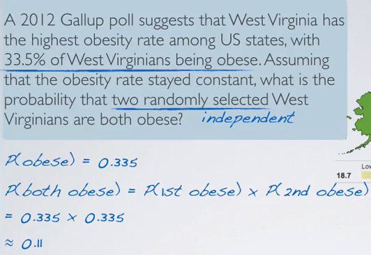

Let's take an example:

Screenshot taken from Coursera video, 01:17

From this example we can get some interesting information. If often useful that, in a lot of question, we're extracting some useful formation in a context of mathematical formula.

We can pick the probability of being obesed is 33.5%. By asumming the that obesity rate stays constant, means that it doesn't change overtime, equals to what we get if we pick them at the same time. Two randomly selected make stronger evidence that this is independent. If it picked in a same household, then it will likely dependendat, as both may share the same food and sports activity.

The probability results than as a given. Note that there's two advantage for calculating the probability:

• Mathematical formula should prove that the product of less than 1 will be smaller.
• It can provide sanity check of your data, if you want to provide some additional practical probability to prove this. It does create advantage if you can design some mathematical formula to prove to your research results.

The Probability Examples

Screenshot taken from Coursera video, 01:17

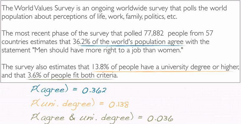
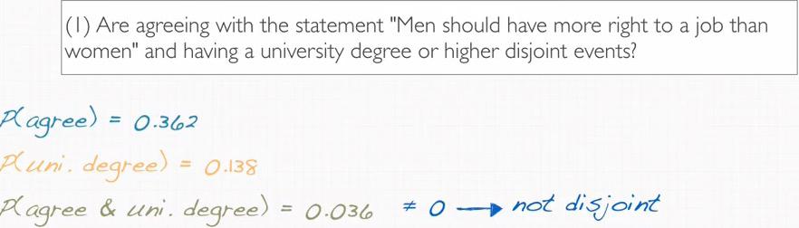
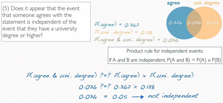
In this case, again we listed all useful information that we get from the stories. We have the probability of 'agree' from the population. We have 13.8% of uni degree. And the intersection between the two. Note that absolute value here, the number of people isn't our concern since we're given relative frequency by percentage, and questions that we want to ask is not about absolute value.

Screenshot taken from Coursera video, 01:17

Since we are hinted at the intersection probability of two events, this two events are not disjoint events. Both events can happen at the same time.

Screenshot taken from Coursera video, 01:17

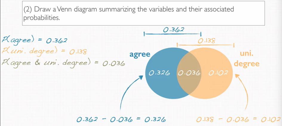
To simplify the problem, we're gonna make a Venn diagram to visualize our problem. Doing this can make two advantage. First we can have easier understanding about the problem if we create a visualization. Second it will becomes as alternative calculation for our questions.

Screenshot taken from Coursera video, 04:28

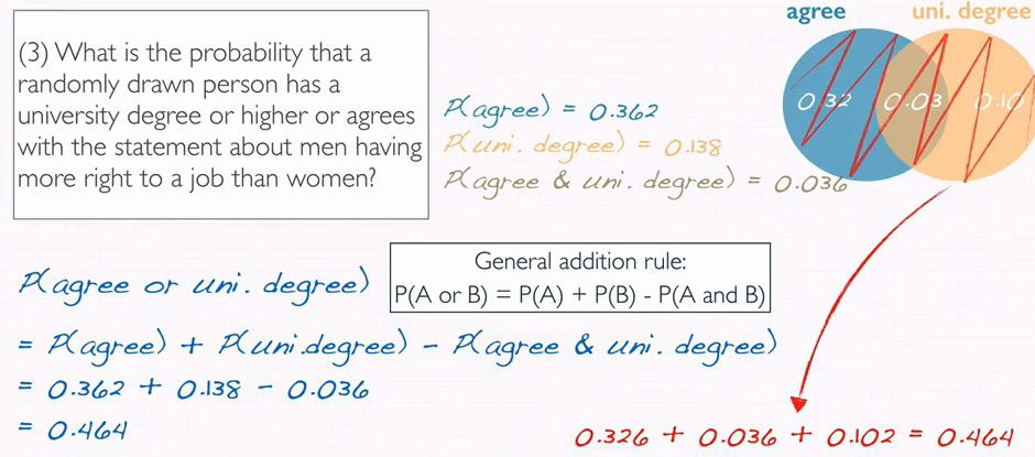
To solve these question, we can proceed with two options:

• Calculate the results by using disjoint events formula. This will sum two events and subtract the intersection
• Using Venn diagram that we create earlier, summing all of the probability since we already get rid of the double counting(the intersection events).

Screenshot taken from Coursera video, 05:08

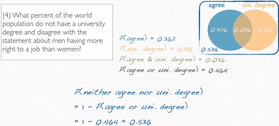
The probability that it's asking is the probability of not A nor B happen. In this case, we can use complementary events, that is outside probability of all the probability events inside both our circle.

Screenshot taken from Coursera video, 06:07

Screenshot taken from Coursera video, 06:07

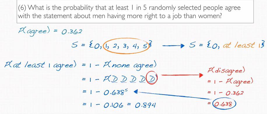
The probability of at least one agree, is the complementary events of all people disagree. Think about it. At least one people agree is higher probability than all 5 people disagree. Then we just take the highest probability which one people agree.

Complementary of all people disagree is the answer we're looking for. If one people agree, or two people agree, or more is the complementary, the sum of the rest probability, of observed event all people disagree.

Disjoint vs Independent

Screenshot taken from Coursera video, 02:27

Remember disjoint is about the the event which can't happen at the same time.Disjoint events can't happen at the same time. Using this provide critical information, that is because "can't happen at the same time", give indication that when first occurs the others can't occurs. This means that disjoint events are dependant.

Independent is that event that provide no useful information to the other event.

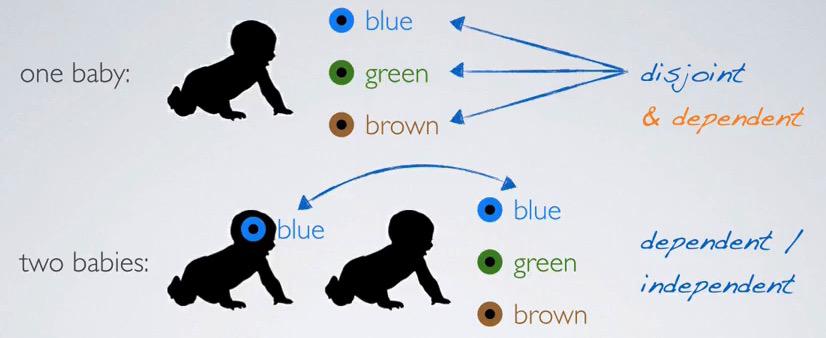
Looking at the baby's color eye example. When observing one baby, if the baby blue, he can't have other colors. This means it provide useful information, that baby has blue eye color.

When we take two or more observed baby, then it becomes independent/dependant choice. If the baby is related or sibling, then it will be dependant of two events occurs. But if two babies are randomly selected from the population, then it will be independent events.

Looking at the coin toss example, one coin toss will be dependant events, since head and tail are disjoint events, comes out head can't be comes out tail at the same time.Two coin toss is independent. First toss will not provide useful information for the second toss.

Conditional Probability

Screenshot taken from Coursera video, 01:15

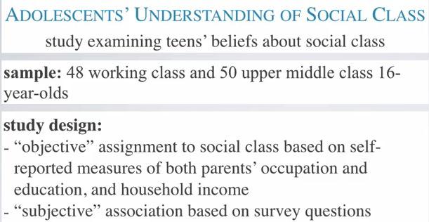
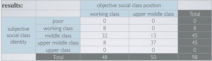
Study taken to include students in a survey, where by objective behind the scenes, the research has collected some information to determine whether the sudents is working class or upper middle class. Then students fills a survey to subjectively determine their own social class.

Screenshot taken from Coursera video, 02:19

Marginal Probability

Marginal probability is the probability that comes incorporating the total. Here's because the question to ask is marginal probability of objective upper class, we're simply take proportion of objective upper class divided by total class.

The objective upper class will be the total of all objective upper class, which is:

$$P(obj UMC) = 50/98 \approx 0.51$$

The subjective upper middle class is:

$$P(obj UMC) = 45/98 \approx 0.46$$

The probability of students that both meet criteria subjective and objective of upper middle class.

$$ P(obj UMC \& subj UMC) = 37/98 \approx 0.38 $$

We also can draw a Venn Diagram which put 37 in the intersection, 8 in subjective UMC, and 13 in objective UMC.

Conditional Probability

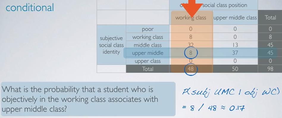
Screenshot taken from Coursera video, 04:29

Conditional Probability is a probability that are given first in the condiion of the first events.

Here if we look at the question, first we're looking at the objective working class, and select those subjective that are associates with upper middle class. Which in turn, given obj WC, which total of 48, select 8 of those. That will calculates the resulting probability.

The probability of students' given subjective upper middle class, which associates with objective upper middle class is:

$$ P(subj MC \mid obj UMC) = 13/50 \approx 0.26$$

The fact that we already have contigency table, simplify our calculation for calculating all the probability.

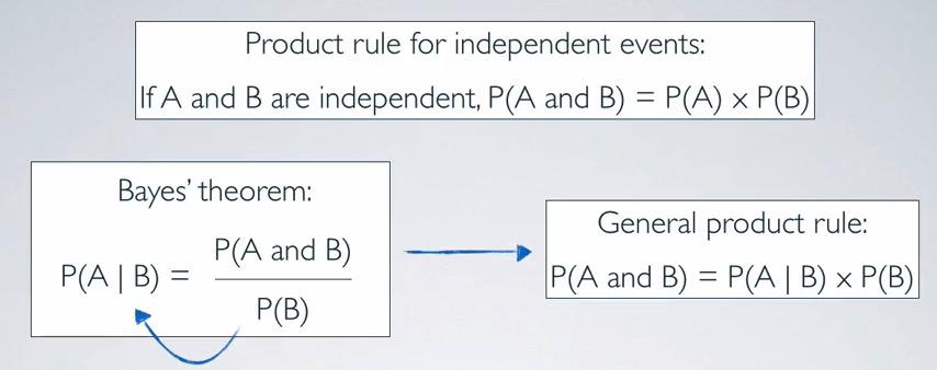
Bayes' theorem

Bayes can be used to solve this question. The formula is

$$ P(A | B) = \frac{P(A and B)} {P(B)}$$

Where the denominator is the probability which we are condition on, the numerator is the joint probability.

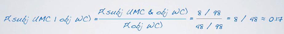
Screenshot taken from Coursera video, 06:15

Screenshot taken from Coursera video, 08:56

Here we take the Bayesian to answer earlier question. This calculation is a little bit overkill because we alredy have the table. But if we don't have that, the Bayesian can calculate it for us.

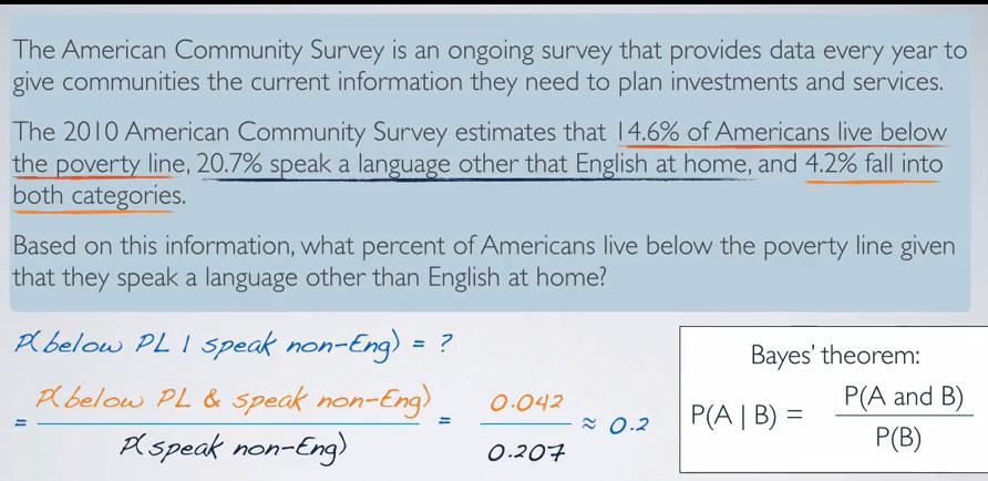
Here's another example that in this case we don't have contigency table. To calculate it, using Bayes' theorem, we arrive at conclusion that roughly 20% of the speak non-Eng live below property line.

In this results, 20% out of all people that speaks other than English live below poverty line. 14.6% out of all people live below in poverty lines, which suggest there's maybe dependant probability of two events.

If we're taking it backward, then out of all people live below povertly line, that also speaks other English is:

$$P(speak non-Eng \mid below PL) = \frac{P(below PL \& speak non-Eng)} {P(speak non-Eng)} = \frac{0.042}{0.146} \approx 0.29$$

Screenshot taken from Coursera video, 09:36

Screenshot taken from Coursera video, 11:00

If we don't know the joint probability but not bayes probability, we can shuffle the formula and arrive at above conclusion.

These are additional rules for proving whether the two events are independent or not. We can use Bayes' theorem and solve it by conceptually or mathemathically.

Here we have another contigency table that provide an example of independent event

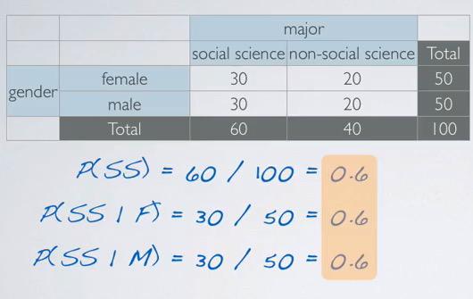
Screenshot taken from Coursera video, 12:39

If we look briefly at the contigency table, where we have each of the total sum up to total of both events, we can see that the events are dependant. By proving it with Bayes's theorem, which resulting same probability of social class, regardless the gender, the gender and the major are independent events.

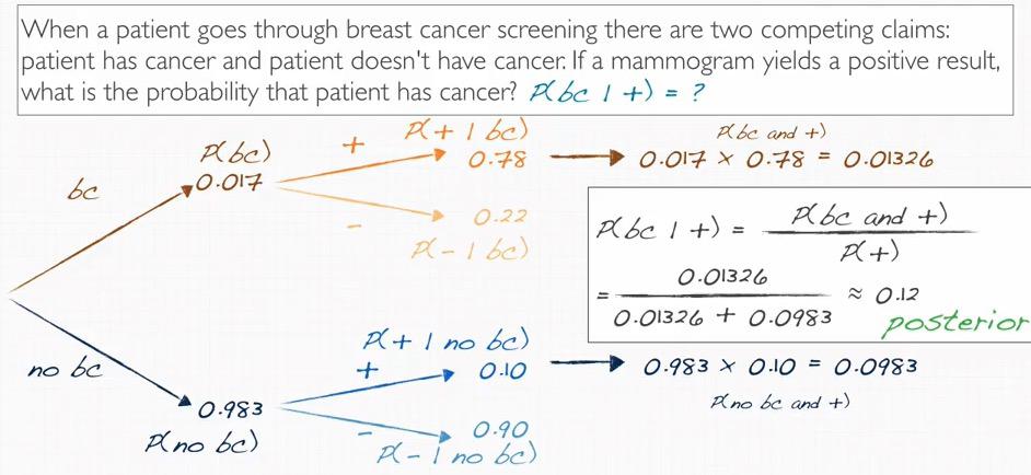
Probability Tree

PT is useful to checking reverse conditional probability.Take a look at this example, when you have absolute number of population.

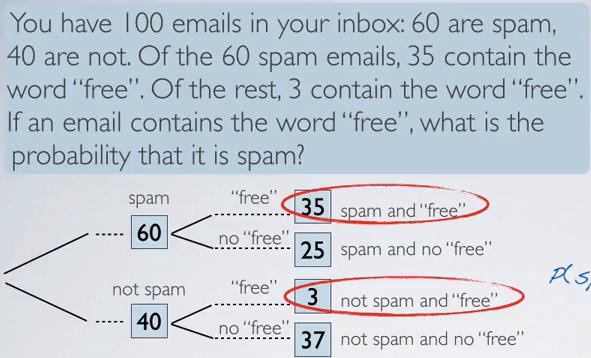
Screenshot taken from Coursera video, 02:48

Here we can use Bayes theorem to solve this problem. Pay attention to the question that we really want to ask, since often it fails because of misunderstanding of the practioners. The question formulates to given 'free', what are the 'spam':

This question will translate to:

$$ P(spam \mid "free") = \frac{35}{35+3} \approx 0.92$$

Here we have another example that only give relative percentage.

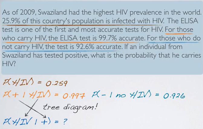
Screenshot taken from Coursera video, 05:07

Here we can prove whether the test accuracy given real HIV/nonHIV. If the events are independent, the resulting probability should be the same. But in this case, P(+ | HIV) $\neq$ P(-|non-HIV) which tells us that this is dependant event.

0.259 HIV     -- 0.997 positive
              -- 0.003 negative
0.741 non-HIV -- 0.074 positive
              -- 0.926 negative

Here's the more complete explanation of the probability tree.

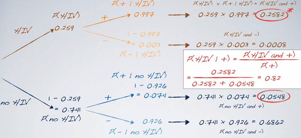
Screenshot taken from Coursera video, 10:07

This results, shows that roughly 82% chance that tested positive have a HIV.

Bayesian Inference

To explain in Bayesian Inference, we use 4 die and 12-die and set a game. The game only tells you provided that you choose either dice(you won't know which die) tells you that either more or less than 4. To explain more intuitively:

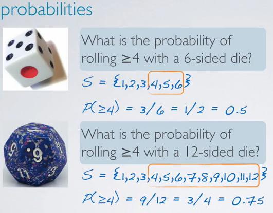
Screenshot taken from Coursera video, 1:37

The rule is that 6-die assigned to one hand side, and 12-die assigned to the other side. You can ask to roll a die, and yes/no question will comes out, either the resulting value comes out greater or nor than 4. There's a tradeback for the game, is that everytime you ask to roll, it costs money. This resembles the world problem that data cost money, larger data need larger resources.Your goal is to find the good die, and guess where the good die reside in which side of the hand.

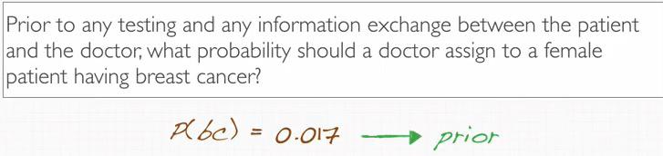
Before you ask to roll the die and collect any dat, both hands has equal chance, 50:50. Suppose we assigned hypothesis as follows:

H1 : good die on the right H2 : bad die on the right

This probabilities is often called prior, we call that because you don't have any information to back up your probability guess.

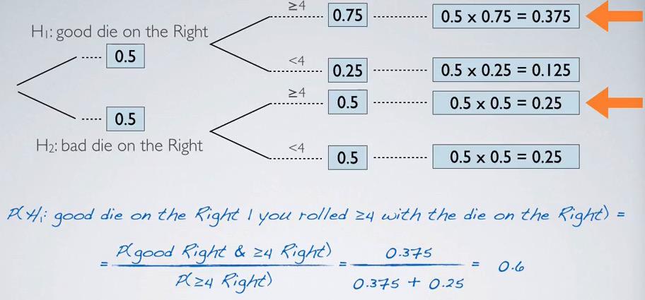
Screenshot taken from Coursera video, 11:17

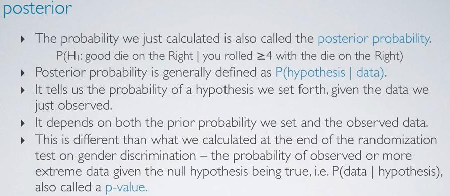
Round #1 : Turns out right hand spits greater than 1.We use probability tree and Bayes' theorem to solve our problem. The posterior probability, the probability after we gain information, should be as we expect, larger than 0.5.The posterior takes stronger ground in this rules.

Screenshot taken from Coursera video, 12:15

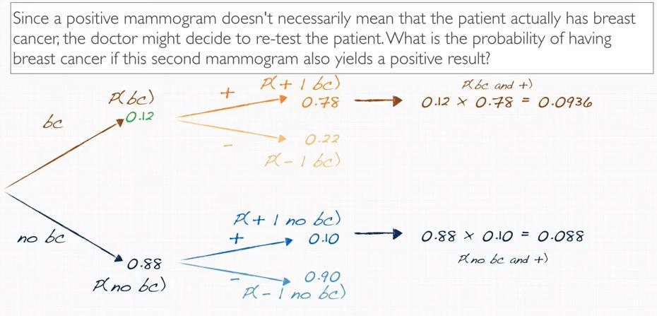
The posterior will serve as our modal to create another prior in the next steps. This give us more and more probability, as we make iterative steps, converges to actual probability.

Screenshot taken from Coursera video, 12:56

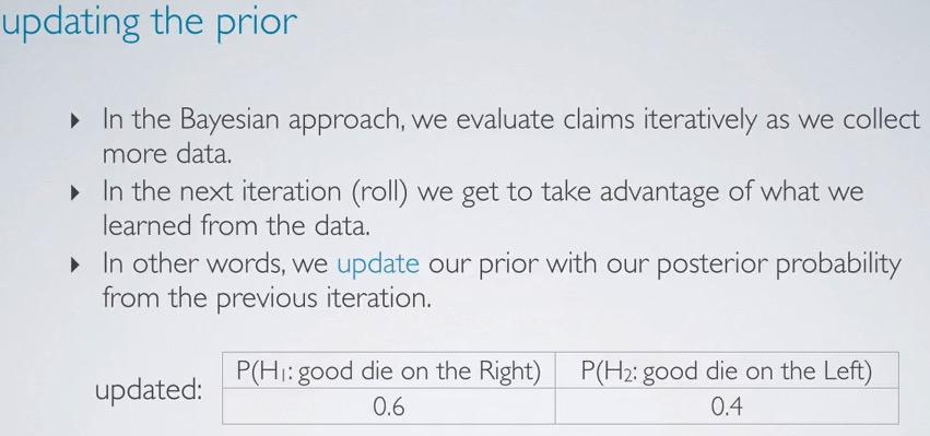
After we have our posterior probability, in the next step we're updating our prior probability to have 0.6 chance of good die being in the right, and complementary probability in the left. Again we request for more roll, and calculate posterior probability and again, updating our prior.

The Bayesian iterative steps is making repetitive of these steps:

updating prior->calculating posterior->updating prior

So how many steps do we need to make a guess? Do we have to wait until the our hypothesis reach 1? There's still fair chance that H2 is true, in this case, we can't wait the prior to finally get 1. It's up to us deciding what are the threshold faith probability. Do we want our probabilty to gain 80% confidence? 95% confidence? Remember that converging to 1 requires extra money, which you should pay attention to that.

Screenshot taken from Coursera video, 14:14

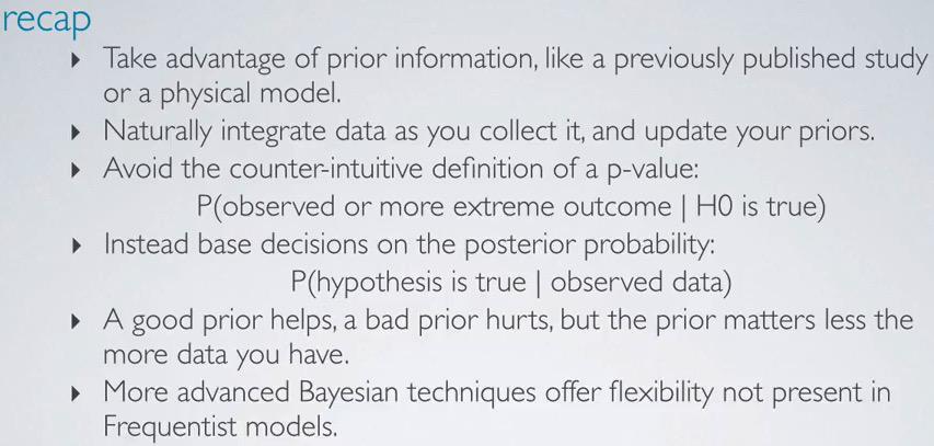
This is a recap conclusion of what we just learn in Bayesian Inference. We take a more and more polished model as we calculate to update our prior probability. Note that prior probability can be any of your choice. But to make more fair prior values, we make educated guess, that in the beginning, all events should served equal chance.As we gain more data, our guess should matter less and less, as our probability will converges to actual probability.

The Bayesian Inference should be not mistaken as p-value, where Bayes steps is to take more and more iterative steps to converge to actual probability, where p-value is taking one steps and observe the probability in extreme conditions given the Null Hypothesis is true.

Here's another example using Bayesian Inference.

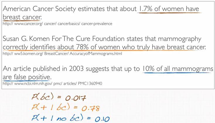
Screenshot taken from Coursera video, 01:02

Screenshot taken from Coursera video, 01:32

Screenshot taken from Coursera video, 01:32

Screenshot taken from Coursera video, 07:12

So finally after our examples before, our iterative steps include:

• setting a prior
• collecting data
• obtaining a posterior
• updating the prior with the previous posterior

REFERENCES:

• https://class.coursera.org/statistics-003/