Support Vector Machine with scikit-learn
SVM(Support Vector Machine) is really popular algorithm nowadays. It's really young but it's fenomenal and use by many. In here we learn why SVM is so powerful. There's also many of SVM blog that i made in the past. If you're curious, please click tag 'Support Vector Machine' at the top of the page.
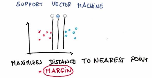
SVM choose the line that maximize the distance of both nearest point. This distance often called Margin.SVM tries to maximize the margin, but also act as other learning algorithm, prioritize the correctness of classifying. Even if there's point that can't be classfied correctly, while retain its largest margin, SVM will treat it as outliers, and can safely ignore the points. But the percentage in which the SVM has firm belief to retain the largest margin, is something called C. Check here to get more intuition about it.
Using SVM with SKlearn

It's really just use the same syntax. We're going to have input,output,fit and predict.
%load '../naive_bayes/class_vis.py'


#!/usr/bin/python

#from udacityplots import *
import matplotlib
matplotlib.use('agg')

import matplotlib.pyplot as plt
import pylab as pl
import numpy as np

#import numpy as np
#import matplotlib.pyplot as plt
#plt.ioff()

def prettyPicture(clf, X_test, y_test):
    x_min = 0.0; x_max = 1.0
    y_min = 0.0; y_max = 1.0

    # Plot the decision boundary. For that, we will assign a color to each
    # point in the mesh [x_min, m_max]x[y_min, y_max].
    h = .01  # step size in the mesh
    xx, yy = np.meshgrid(np.arange(x_min, x_max, h), np.arange(y_min, y_max, h))
    Z = clf.predict(np.c_[xx.ravel(), yy.ravel()])

    # Put the result into a color plot
    Z = Z.reshape(xx.shape)
    plt.xlim(xx.min(), xx.max())
    plt.ylim(yy.min(), yy.max())

    plt.pcolormesh(xx, yy, Z, cmap=pl.cm.seismic)

    # Plot also the test points
    grade_sig = [X_test[ii][0] for ii in range(0, len(X_test)) if y_test[ii]==0]
    bumpy_sig = [X_test[ii][1] for ii in range(0, len(X_test)) if y_test[ii]==0]
    grade_bkg = [X_test[ii][0] for ii in range(0, len(X_test)) if y_test[ii]==1]
    bumpy_bkg = [X_test[ii][1] for ii in range(0, len(X_test)) if y_test[ii]==1]

    plt.scatter(grade_sig, bumpy_sig, color = "b", label="fast")
    plt.scatter(grade_bkg, bumpy_bkg, color = "r", label="slow")
    plt.legend()
    plt.xlabel("bumpiness")
    plt.ylabel("grade")

    plt.savefig("test.png")

import base64
import json
import subprocess

def output_image(name, format, bytes):
    image_start = "BEGIN_IMAGE_f9825uweof8jw9fj4r8"
    image_end = "END_IMAGE_0238jfw08fjsiufhw8frs"
    data = {}
    data['name'] = name
    data['format'] = format
    data['bytes'] = base64.encodestring(bytes)
    print image_start+json.dumps(data)+image_end


%load '../naive_bayes/prep_terrain_data.py'


#!/usr/bin/python
import random


def makeTerrainData(n_points=1000):
###############################################################################
### make the toy dataset
    random.seed(42)
    grade = [random.random() for ii in range(0,n_points)]
    bumpy = [random.random() for ii in range(0,n_points)]
    error = [random.random() for ii in range(0,n_points)]
    y = [round(grade[ii]*bumpy[ii]+0.3+0.1*error[ii]) for ii in range(0,n_points)]
    for ii in range(0, len(y)):
        if grade[ii]>0.8 or bumpy[ii]>0.8:
            y[ii] = 1.0

### split into train/test sets
    X = [[gg, ss] for gg, ss in zip(grade, bumpy)]
    split = int(0.75*n_points)
    X_train = X[0:split]
    X_test  = X[split:]
    y_train = y[0:split]
    y_test  = y[split:]

    grade_sig = [X_train[ii][0] for ii in range(0, len(X_train)) if y_train[ii]==0]
    bumpy_sig = [X_train[ii][1] for ii in range(0, len(X_train)) if y_train[ii]==0]
    grade_bkg = [X_train[ii][0] for ii in range(0, len(X_train)) if y_train[ii]==1]
    bumpy_bkg = [X_train[ii][1] for ii in range(0, len(X_train)) if y_train[ii]==1]

#    training_data = {"fast":{"grade":grade_sig, "bumpiness":bumpy_sig}
#            , "slow":{"grade":grade_bkg, "bumpiness":bumpy_bkg}}


    grade_sig = [X_test[ii][0] for ii in range(0, len(X_test)) if y_test[ii]==0]
    bumpy_sig = [X_test[ii][1] for ii in range(0, len(X_test)) if y_test[ii]==0]
    grade_bkg = [X_test[ii][0] for ii in range(0, len(X_test)) if y_test[ii]==1]
    bumpy_bkg = [X_test[ii][1] for ii in range(0, len(X_test)) if y_test[ii]==1]

    test_data = {"fast":{"grade":grade_sig, "bumpiness":bumpy_sig}
            , "slow":{"grade":grade_bkg, "bumpiness":bumpy_bkg}}

    return X_train, y_train, X_test, y_test
#    return training_data, test_data


import sys
from class_vis import prettyPicture
from prep_terrain_data import makeTerrainData

import matplotlib.pyplot as plt
import copy
import numpy as np
import pylab as pl


features_train, labels_train, features_test, labels_test = makeTerrainData()


########################## SVM #################################
### we handle the import statement and SVC creation for you here
from sklearn.svm import SVC
clf = SVC(kernel="linear")


#### now your job is to fit the classifier
#### using the training features/labels, and to
#### make a set of predictions on the test data

clf.fit(features_train,labels_train)


#### store your predictions in a list named pred

pred = clf.predict(features_test)


from sklearn.metrics import accuracy_score
acc = accuracy_score(pred, labels_test)

def submitAccuracy():
    return acc
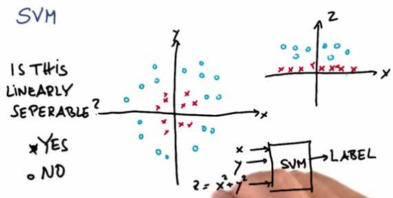
SVM will gives us linear separable if we're trying to include polynomial features if we're trying to solve non-linear data. The z features, as two dimensional, will consider the problem as top right, making z capable of linearly separating the graph.
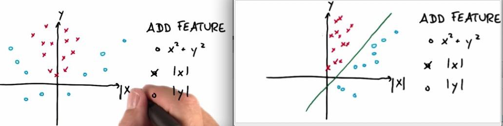
Adding |x| as new feature, will flip all the point in -x into x+.Which in turn makes the graph linearly separable.
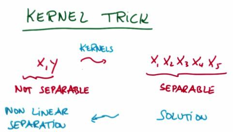
There's kernel trick to create x parameter to become more polynomial. Check this link for more intuition
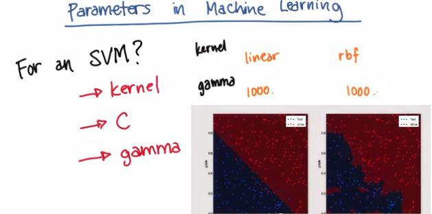
It's important to understand more of parameters in SVM
Please check the sklearn for more documentation in this link
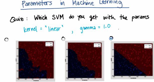
import sys


%pylab inline

Populating the interactive namespace from numpy and matplotlib


sys.path.append('../naive_bayes')


import sys
from class_vis import prettyPicture
from prep_terrain_data import makeTerrainData

import matplotlib.pyplot as plt
import copy
import numpy as np
import pylab as pl


features_train, labels_train, features_test, labels_test = makeTerrainData()


from sklearn.svm import SVC


clf = SVC(kernel='linear',gamma=1.0)


clf.fit(features_train,labels_train)


SVC(C=1.0, cache_size=200, class_weight=None, coef0=0.0, degree=3, gamma=1.0,
  kernel='linear', max_iter=-1, probability=False, random_state=None,
  shrinking=True, tol=0.001, verbose=False)


prettyPicture(clf, features_test, labels_test)

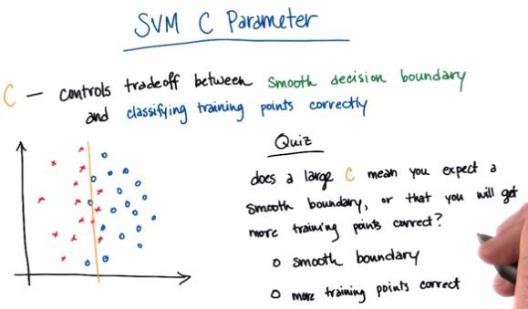
For this quiz, the answer should me more training corrects. C works as contrary of lambda, where the larger the C, the more the system overfit the train data. Again, you may check at this link to get more intuition about C value.
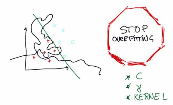
The Machine Learning nightmare is overfitting. Anything can happen, if not optimal, then you either get underfitting or overfitting. This also take into account that all of these 3, if not tuned correctly will be prone to overfitting.
Final Thoughts
SVM can be at an advantage and disadvantage. If we can see clear distance separable plane between two datasets, then it's a good idea to use SVM. But, because SVM has firm belief(shown by 'margin'), it has weakness in datasets that have close margin. For this, Naive Bayes is recommended.
It also tends to not work so well given huge dataset and huge parameters. It still good, but the algorithm will be very slow. For this, there's many library implementing SVM have readily optimize SVM. For more thoughts into this, please check this link
Mini Project
In this mini-project, we’ll tackle the exact same email author ID problem as the Naive Bayes mini-project, but now with an SVM. What we find will help clarify some of the practical differences between the two algorithms. This project also gives us a chance to play around with parameters a lot more than Naive Bayes did, so we will do that too.
%load svm_author_id.py


#!/usr/bin/python

"""
    this is the code to accompany the Lesson 2 (SVM) mini-project

    use an SVM to identify emails from the Enron corpus by their authors

    Sara has label 0
    Chris has label 1

"""

import sys
from time import time
sys.path.append("../tools/")
from email_preprocess import preprocess


### features_train and features_test are the features for the training
### and testing datasets, respectively
### labels_train and labels_test are the corresponding item labels
features_train, features_test, labels_train, labels_test = preprocess()


no. of Chris training emails: 7936
no. of Sara training emails: 7884


clf = SVC(kernel='linear')


clf.fit(features_train,labels_train)


SVC(C=1.0, cache_size=200, class_weight=None, coef0=0.0, degree=3, gamma=0.0,
  kernel='linear', max_iter=-1, probability=False, random_state=None,
  shrinking=True, tol=0.001, verbose=False)
And the accuracy of this classifier is....
clf.score(features_test,labels_test)


0.98407281001137659
exact times may vary a bit, but in general, the SVM is MUCH slower to train and use for predicting
features_train = features_train[:len(features_train)/100]
labels_train = labels_train[:len(labels_train)/100]


clf.fit(features_train,labels_train)


SVC(C=1.0, cache_size=200, class_weight=None, coef0=0.0, degree=3, gamma=0.0,
  kernel='linear', max_iter=-1, probability=False, random_state=None,
  shrinking=True, tol=0.001, verbose=False)


clf.score(features_test,labels_test)


0.88452787258248011
Only 1% of the features, but over 88% the performance? Not too shabby!
It's good sometimes to have lower performance but instance learning. Voice recognition and transaction blocking need to happen in real time, with almost no delay. There's no obvious need to predict an email author instantly.
clf_rbf = SVC(kernel='rbf')


clf_rbf.fit(features_train,labels_train)


SVC(C=1.0, cache_size=200, class_weight=None, coef0=0.0, degree=3, gamma=0.0,
  kernel='rbf', max_iter=-1, probability=False, random_state=None,
  shrinking=True, tol=0.001, verbose=False)


clf_rbf.score(features_test,labels_test)


0.61604095563139927
C (say, 10.0, 100., 1000., and 10000.). Which one gives the best accuracy?
clf_rbf = SVC(kernel='rbf',C=10000)


clf_rbf.fit(features_train,labels_train)


SVC(C=10000, cache_size=200, class_weight=None, coef0=0.0, degree=3,
  gamma=0.0, kernel='rbf', max_iter=-1, probability=False,
  random_state=None, shrinking=True, tol=0.001, verbose=False)


clf_rbf.score(features_test,labels_test)


0.89249146757679176


features_train, features_test, labels_train, labels_test = preprocess()

no. of Chris training emails: 7936
no. of Sara training emails: 7884


clf_rbf.fit(features_train,labels_train)


SVC(C=10000, cache_size=200, class_weight=None, coef0=0.0, degree=3,
  gamma=0.0, kernel='rbf', max_iter=-1, probability=False,
  random_state=None, shrinking=True, tol=0.001, verbose=False)


clf_rbf.score(features_test,labels_test)


0.99089874857792948
Over 99% accuracy, pretty good!
What class does your SVM (0 or 1, corresponding to Sara and Chris respectively) predict for element 10 of the test set? The 26th? The 50th? (Use the RBF kernel, C=10000, and 1% of the training set. Normally you'd get the best results using the full training set, but we found that using 1% sped up the computation considerably and did not change our results--so feel free to use that shortcut here.)
And just to be clear, the data point numbers that we give here (10, 26, 50) assume a zero-indexed list. So the correct answer for element #100 would be found using something like answer=predictions[100]
features_train = features_train[:len(features_train)/100]
labels_train = labels_train[:len(labels_train)/100]


clf_rbf = SVC(kernel='rbf',C=10000)


clf_rbf.fit(features_train,labels_train)


SVC(C=10000, cache_size=200, class_weight=None, coef0=0.0, degree=3,
  gamma=0.0, kernel='rbf', max_iter=-1, probability=False,
  random_state=None, shrinking=True, tol=0.001, verbose=False)


pred = clf_rbf.predict(features_test)


print pred[10]
print pred[26]
print pred[50]

1
0
1
Just like the SVM, you are over 99% correct! (Actually, on this one, you're 100% correct)
features_train, features_test, labels_train, labels_test = preprocess()

no. of Chris training emails: 7936
no. of Sara training emails: 7884


clf_rbf = SVC(kernel='rbf',C=10000)


clf_rbf.fit(features_train,labels_train)


SVC(C=10000, cache_size=200, class_weight=None, coef0=0.0, degree=3,
  gamma=0.0, kernel='rbf', max_iter=-1, probability=False,
  random_state=None, shrinking=True, tol=0.001, verbose=False)


pred = clf_rbf.predict(features_test)


len(pred)


1758


n = []


[n.append(e) for e in pred if e == 1]


len(n)


877
Thoughts on Instructor
Hopefully it’s becoming clearer what Sebastian meant when he said Naive Bayes is great for text--it’s faster and generally gives better performance than an SVM for this particular problem. Of course, there are plenty of other problems where an SVM might work better. Knowing which one to try when you’re tackling a problem for the first time is part of the art and science of machine learning. In addition to picking your algorithm, depending on which one you try, there are parameter tunes to worry about as well, and the possibility of overfitting (especially if you don’t have lots of training data).
Our general suggestion is to try a few different algorithms for each problem. Tuning the parameters can be a lot of work, but just sit tight for now--toward the end of the class we will introduce you to GridCV, a great sklearn tool that can find an optimal parameter tune almost automatically.