Screenshot taken from Coursera 03:42

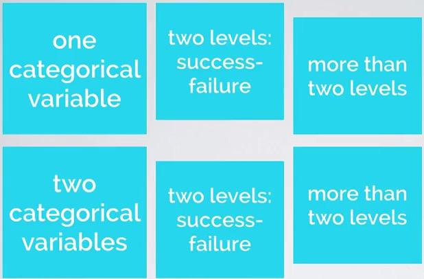
In numerical variable, you want to take the average mean and infer the average and the differences. In categorical variable, you take the proportion of frequency, you may want to perform some contigency table.Studies that take percentage are likely categorical variables (XX% support vs XX% oppose same sex marriage).

In this blog we're going to observe one categorical variable. We talk about binary classification, and then more than two classification. Then we're going to compare two categorical variables, again with binary classification and more than two classification.

Sampling Distribution

Screenshot taken from Coursera 05:10

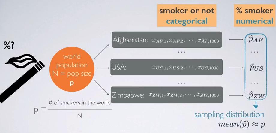
Recall that sampling distribution is when you take infinite times/all possible combination of sample, for particular sample size, and draw the summary statistic from each of the sample distribution and make a distribution out of it.

So for example we observe categorical variable of smoker vs non-smoker. Because we don't know the population proportion and size, we make an estimate on each of the country. We take 1000 sample size for each country and calculate the proportion. The proportions will make a sampling distribution, and the average of proportions will be approximate proportion of whole population. So you see, in the beginning we have categorical variable, but we just observe one levels and convert its sample statistics, which is numerical variables.

Screenshot taken from Coursera 07:20

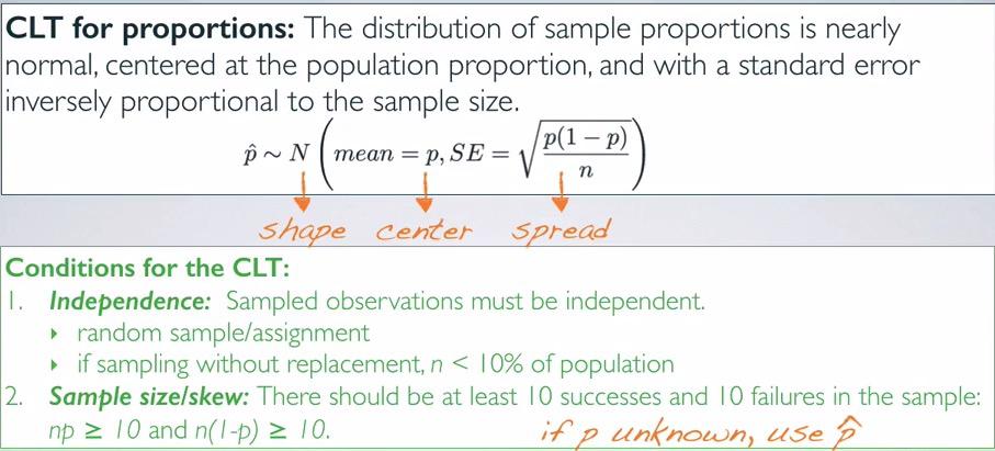
CLT is the same for proportion when use it on mean. From CLT, we want to know shape, center, and spread. The CLT requires us to use random sampling/assignment, and the mean is just equal the proportion. Spread can be calculated by incorporates the proportions and the complements divided by sample size. Then for sample size, this is similar to what we require in binomial, where you have incorporates sample size, success proportion, and failure proportions.So if p population is unknown, use point estimate proportion.

Screenshot taken from Coursera 11:01

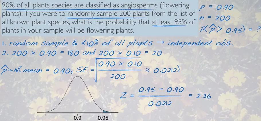
Take a look at this example. We're going to calculate the probability of at least 95% of 200 randomly selected sampled that are flowering plants. That what we usually calculate it before using pnorm function in R. Check the condtitions whether it satisfied the CLT or not. After that, we also want to meet binomial conditions for our sample size. If both conditions satisfied, we can shade the distribution and calculate it by using R what we get is.Remember that we're using least not exact in the distribution,because there's no such thing as cut exact in probability.

pnorm(0.95,mean=0.9,sd=0.0212,lower.tail=F)

[1] 0.009174713

We also can do this in binomial. We know that using binomial, the expected value (mean) is just sample size times probability of success.

n = 200
p = 0.95

n*p

[1] 190

So using just binomial distribution, we're summing up 190 to 200, because we're interested of probability of getting at least 190,

P(190) + P(191) .. + P(200),

sum(dbinom(190:200,200,0.90))

[1] 0.00807125

It's not exactly the same as we previously calculated, but nevertheless look similar.

Screenshot taken from Coursera 15:40

So what if the success-failure (np > 10 && n(1-p) > 10) conditions are not met?

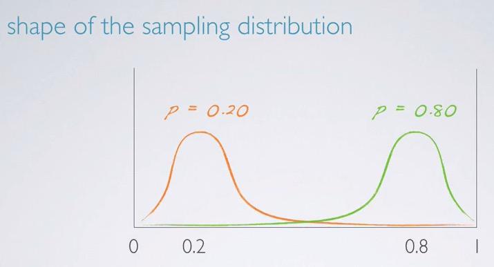
The center of sampling distribution will be around at the population proportion. You see that we have 0 and 1 boundary. This is intuitive, as there are no >100% proportion or < 0% proportion. So we have those boundary. We have one proportion that closer to zero, and we also have proportion that closer to one. You see that sampling distribution is centered around the proportion of the sample.

The spread can be calculated using standard error formula. We have proportion, proportion complements and sample size.

But the shape is what differs. When the proportion is closer to zero, like 0.20 in the example, we have natural boundary of the distribution can't be less than 1, this will make a long tail towards 1. Same goes for propotion that in 0.8. So depending on the propotion, we can have skewed distribution.

Intuitively, using previous examples when we have 50 random sample, 90% of p will gives us left skewed distribution.

Confidence Interval

Screenshot taken from Coursera 01:38

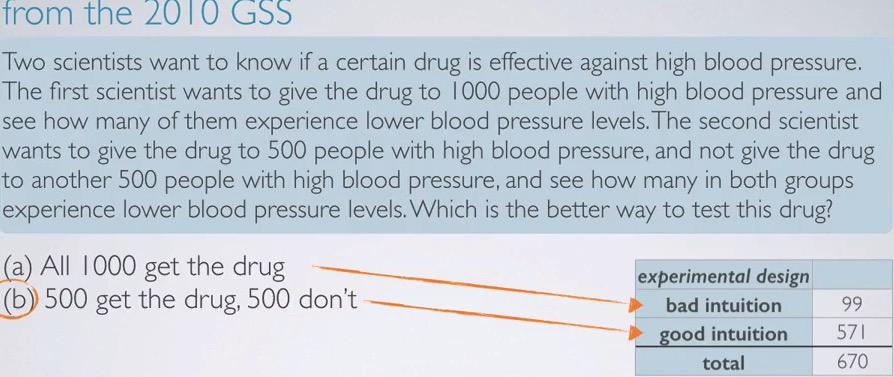
Don't try to focus on this question, it's just act as a basis of next research question. So we're know that controlling is a better study design, we divided into treatment and control groups, so b is a better choice. This question asked to 670 people and we focus on the proportion.

Screenshot taken from Coursera 02:17

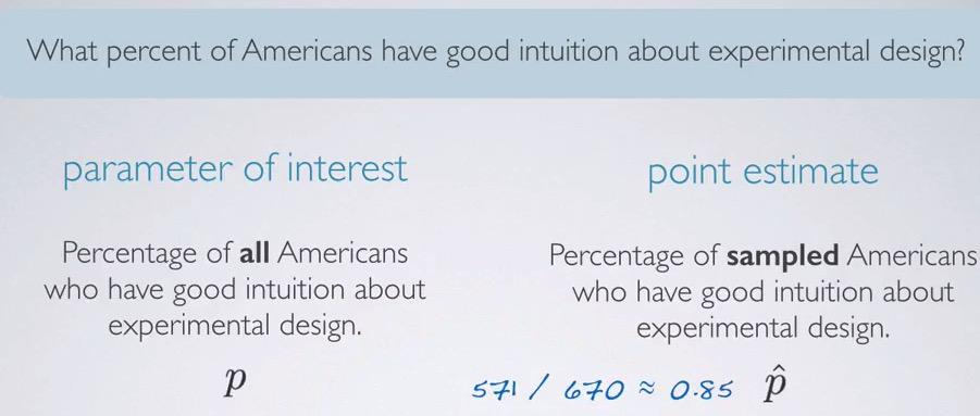
So we want to estimate the proportion of population, as parameter of interest. The point estimate is what we can calculate using our sample.

Screenshot taken from Coursera 09:59

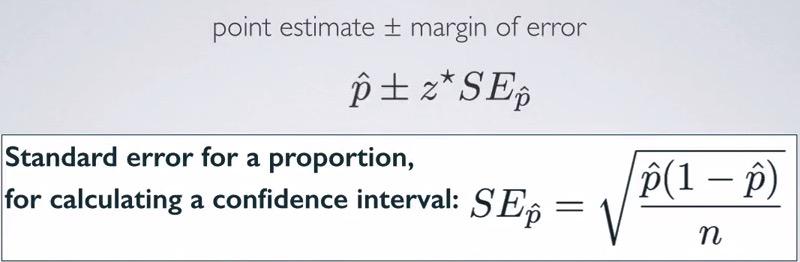
So before, we calculate the standard error of population proportion. But we also know that it's almost not available.So what we can do is get the standard error of point estimate proportion.

So how do you calculate the confidence interval? Use 95% confidence level.

First check the conditions

• Independence. We know that 670 is less than 10% population, and GSS is sampling randomly. So we know that one sampled of American has good intuition about experimental design will be independent of one another.
• Sample size/skewness. For the sample size, we can use formula to assert the enough sample size. But actually we can eyeballing by looking at the example. we have 571 successes and 99 failures, and both are greater than 10. So failures and successes are met, so we know that our sampling distribution will be nearly normal.

p = 0.85
n = 670
CL = 0.95
SE = sqrt(p*(1-p)/n)
z_star = round(qnorm((1-CL)/2,lower.tail=F),digits=2)
ME = z_star * SE

c(p-ME, p+ME)

[1] 0.822962 0.877038

So based on this data, we can interpret confidence interval as:

• We are 95% confident that 83% to 87% of all Americans have good intuition about experimental design.
• 95% of random samples of 670 Americans will yield confidence interval that will capture true proportion of Americans that have good intuition about experimental design.

Required sample size of desired ME

Screenshot taken from Coursera 08:41

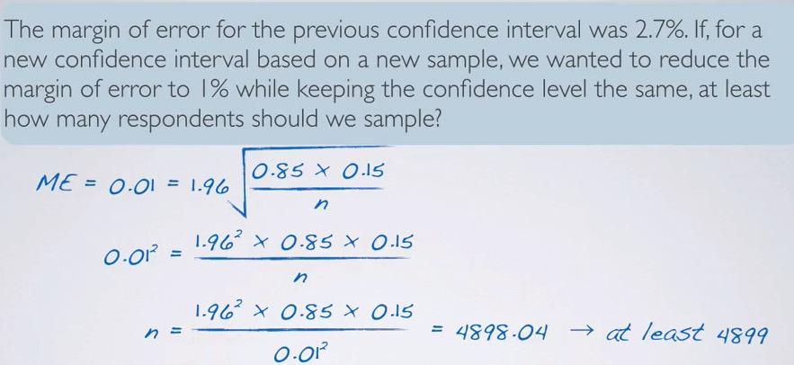
So we previously learned about required sampled size for point estimate mean. For categorical variable, we use manipulate the parameter in standard of error. Since this is same example, we're going to use same proportion. Specifying the desired ME, and leave n for final calculations, we get the results. Since this is the threshold of minimal requirements, .04 will be round up 1, since there are .04 person(numerical discrete)

#Required sample size proportion for desired ME

p = 0.85
z_star = 1.96
ME = 0.01

z_star**2*p*(1-p)/ME**2

[1] 4898.04

If we have $\hat{p}$, we can use the value to put into our calculations. If we don't have it, we use 0.5. This is picked for two reasons

• 50:50 is best estimate (prior) for one categorical variable with two levels.
• 0.5 will give us the largest possible sample size.

Screenshot taken from Coursera 09:27

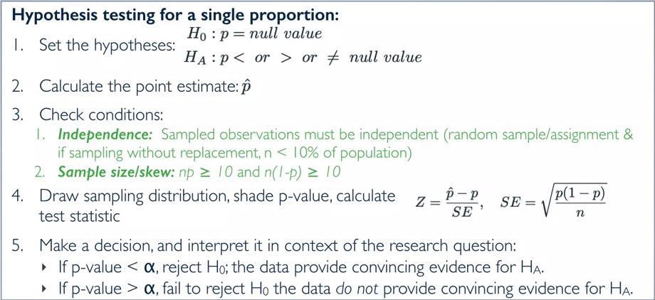
HT framework is also applies really similar to what we do in the mean.

First we set null and alternative hypothesis test. Remember that we use population parameter, like in CI, because they both want to infer the population parameter. What you have in this data, will reject or fail to reject the null hypothesis.

We set our point estimate as proportion sampled.

We check the conditions. Similar to mean we want to have less than 10% population and random sample/assignment. But the diference is when you have larger than 30 for mean, you want to have larger than 10 successes and larger than 10 failures. This is the expected value like in the binomial, so p will be picked, instead of p hat.

Draw the sampling distribution and shade p-value are (ALWAYS). calculate the Z critical, again we use the proportion for our SE(always when available).

Finally we make a decision, if it smaller than the threshold, reject null hypothesis. Otherwise we fail to reject null hypothesis.

Screenshot taken from Coursera 04:33

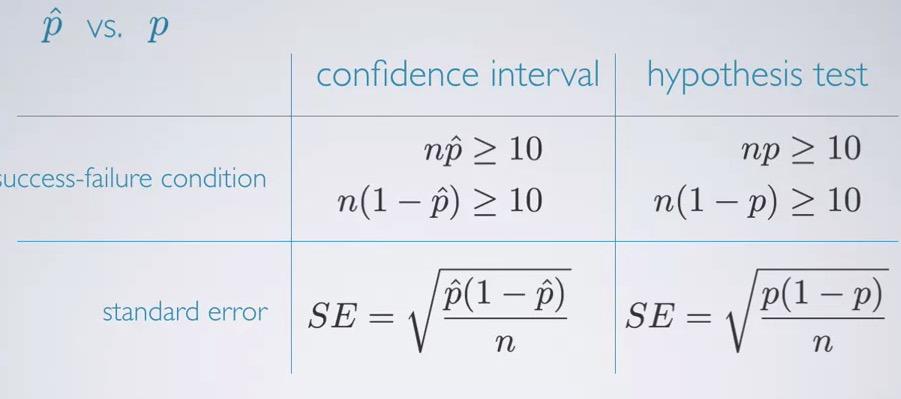
So there notice any difference that you have between CI and HT. When you in CI, you calculate the proportion and range of difference. When you're in HT, you're given the null value, the true proportion of the population. So you use that instead. We're always using true proportion whenever possible. In CI case, the true proportion is unknown so we use the point estimate. in HT, because true proportion is given (as null value), we calculate the failures,successes, and SE based on null value.

Screenshot taken from Coursera 07:00

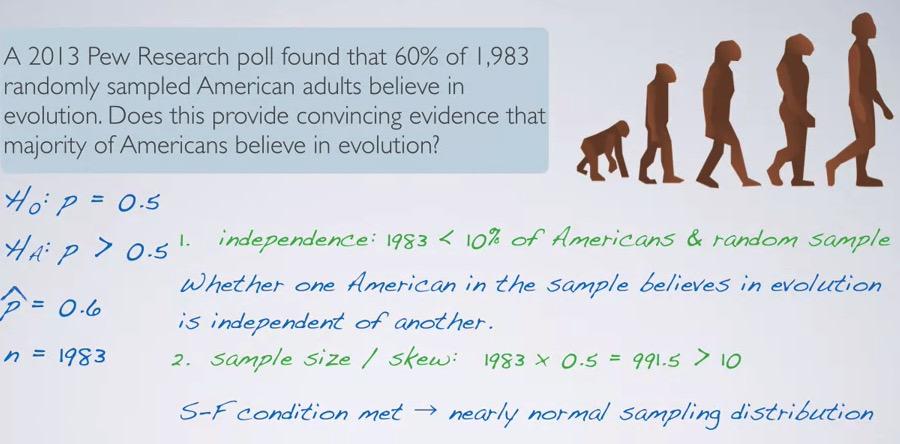
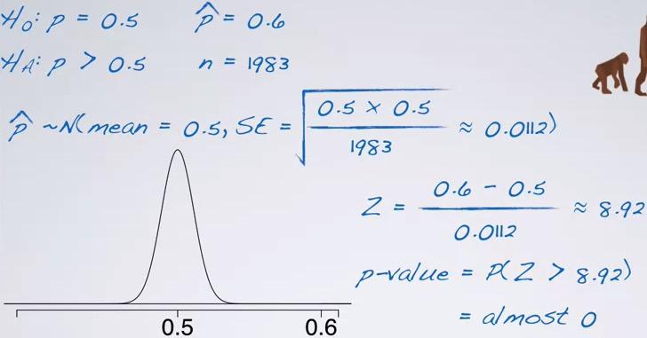
Here in the example we want to use hypothesis test to know whether the majority of the Americans believe in evolution. Majority will be whichever proportion that are greater than 50%. We want to test it using our given data.

Since the question is about the alternative hypothesis, we can infer the null hypothesis, and we have proportion estimate of 0.6. Then we check the conditions.

1. Independence. 1983 less than 10% population. Whether Americans in sampled believes in population is independent of one another.
2. Sample size/skew. 1983 * 0.5 = 991.5 > 10. We don't have to calculate the complements, because 0.5 applies to both. S-F condition met, we know that sampling distribution will be nearly normal.

After we validate the condition, we now proceed to the next step.

Screenshot taken from Coursera 09:24

#Hypothesis testing, one categorical variable, given null value(p)

p = 0.5
p_hat = 0.6
n = 1983
SL = 0.05
SE = sqrt(p*(1-p)/n)
z_star = round(qnorm((1-CL)/2,lower.tail=F),digits=2)

pnorm(p_hat,mean=p,sd=SE,lower.tail=p_hat < p)

[1] 2.641113e-19

The p-value is practically zero, thus we reject the null hypothesis. There is almost 0% chance that 1983 randomly selected Americans where 60% of them or more believe in evolution, if in fact 50% of Americans believe in population. So the data provide convincing evidence that majority of all Americans believe in evolution.

Summary

When defining population proportion, you use p. When you define sample proportion, you use $\hat{p}$. Plug population proportion to standard error formula. But since it almost always not known, use sample proportion.

For proportion, CLT states that the distribution of sample distribution will be nearly normal, centered at the true population proportion,with standard error as long as:

* Observations in the sample are independent to one another.
* At least 10 expected success and 10 expected failures in the observations.

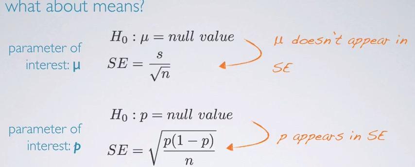
For confidence interval, we use sampled proportion (if we already know the true population proportion, it's useless to build an interval to capture it). For hypothesis testing, we have true population,and incorporate it to our standard error calculation.For numerical variable, standard error doesn't incorporate mean, it uses standard deviation. So it doesn't have discrepancy for computing confidence interval and hypothesis testing.

When calculating required sample size for particular margin of error, if sampled proportion is unknown, we use 0.5. This have advantage in two ways. First, if categorical variable only have two levels, we have fair judgement, best prior uniform. Second, 0.5 will gives us the largest sample size.

Estimating difference between two proportions (confidence interval)

In this section we want to calculate the proportions of each of group in categorical variable.

Screenshot taken from Coursera 04:05

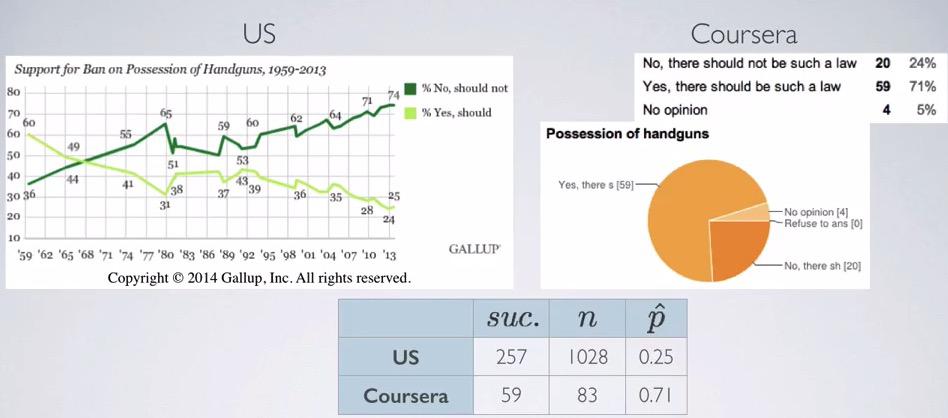
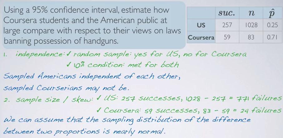
Here we have sample from population, one from Gallup Survey, and the other one from Coursera. The proportion of success is the proportion of citizen that yes, believe there should be law to ban all handgun possesion beside police officer. Here we have different proportion between US and Coursera. It could be that those strong issue that happen in the US, is not so much in the Coursera which consist international students.

Screenshot taken from Coursera 04:19

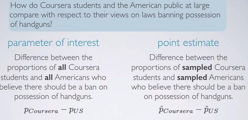
Posted a question, we're making a definition between parameter of interest and point estimate.

Screenshot taken from Coursera 05:55

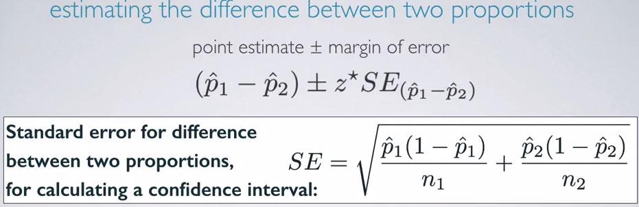
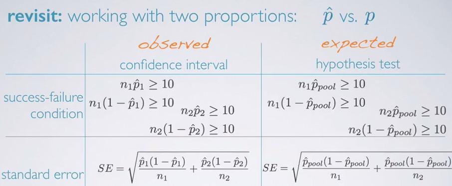
Again we're calculating confidence interval, so we're going the calculate the point estimate difference and standard error difference. Standard error will bigger since we're including variability of both p1 and p2. Mind that we use p hat because population parameter is unknown, later in HT we're going to replace that based on population parameter.

Screenshot taken from Coursera 08:00

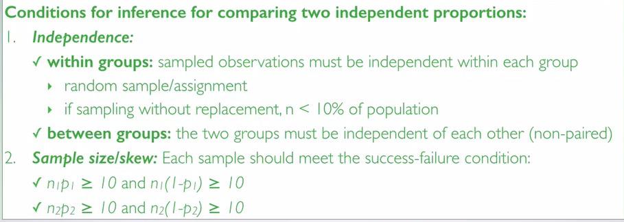
Again the confidence interval of two group must be check.

• Independence. Ensure that within groups must be independent(random sampling/assignment, without replacement < 10% population). And between groups is independent as wel (non-paired).
• Sample size/skew. each of the group must validate success/failure condition (have at least 10 succeses and 10 failures). Remember that we're using proportion sample since proportion population is unknown.

Screenshot taken from Coursera 10:48

So, again we continue the example. Check the conditions.

• Each of the sample size is higher than 10% of their respective population.Gallup survey has doing good joob of random sampling but not for Coursera. their survey is voluntarily survey. So we can say that sampled Americans are independent, sampled Americans may not independent.
• using subtraction on each of the table we have 257 sucesses and 771 failures on US, and 59 succeses and 24 failures on Courserians. Because both of them more than 10, we can say sampling distributions of both proportions are nearly normal.

So let's put it into the equation.

#Observe one level in categorical variable, of categorical of two levels.
#1  = Coursera, 2 = US
n_1 = 83
p_1 = 0.71

n_2 = 1028
p_2 = 0.25

CL = 0.95

SE = sqrt(   (p_1*(1-p_1)/n_1)+(p_2*(1-p_2)/n_2)   )
z_star = round(qnorm((1-CL)/2, lower.tail=F),digits=2)
ME = z_star*SE

c((p_1-p_2)-ME, (p_1-p_2)+ME)

[1] 0.3588534 0.5611466

Since the difference proportion is Coursera-US, we can say that we are 95% confident that proportion of Courserians is 36% to 56% higher than US that believe there should be law for banning gun possesion . Eventhough we change the order, we get same results, and US will be lower than Courserians, which is equals to the statement earlier.

Should we expect significant difference when we do hypothesis testing? Of course! we know that Courserians has 36% to 56% higher than US, then that would means the difference will be significance(compared to null hypothesis, null value is 0% difference). We also know that 0% is not in the (36,56) interval

Screenshot taken from Coursera 02:31

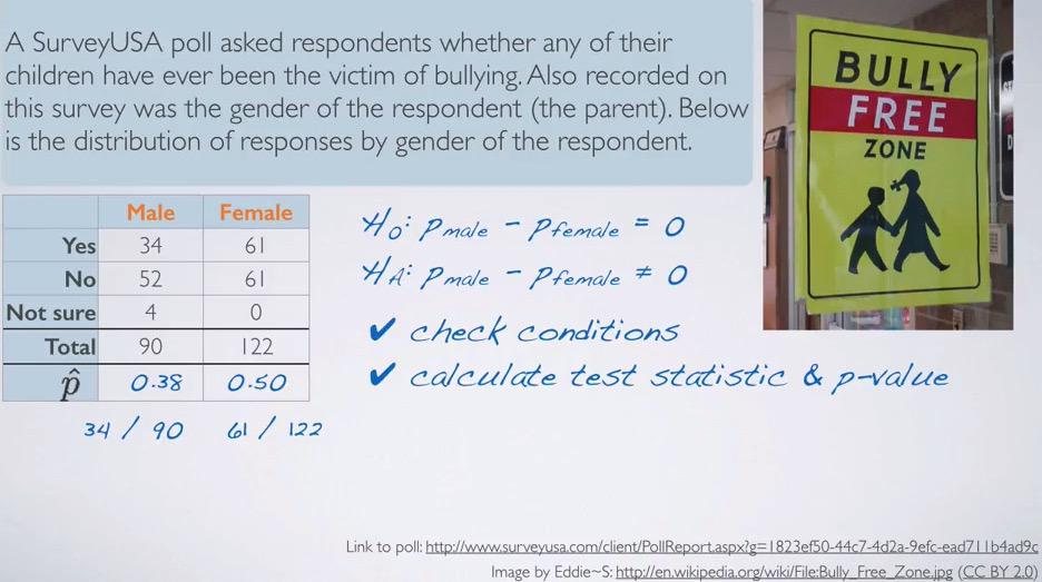
In this example we perform hypothesis test to see the sucess proportions(yes, bullied) between parent that are male/female (only represent by one parent). The null hypothesis there will be no difference,while the alternative state there are a difference. Remember that hypothesis testing is always about the true proportion.In CI, you use observed proportion(if you already know the true proportion, then you shouldn't calculate the interval to capture the the value, because you already know exactly the true proportion).

Remember that for CI we use the observed proportion, but it's little difficult for HT. we don't know the exact value of proportion 1 and proportion 2 equal to. So what do we do? We make one up. The idea is because the proportion is equal, they should be equal proportion if they joined into one population (which is both female and male are two levels of one categorical variable). So what we get is

$$\hat{p}_\mathbf{pool} = \frac{Nsuccess_1+Nsucces_2}{n_1+n_2}$$

calculating p pool we get,

np_1 = 34
np_2 = 61

n_1 = 90
n_2 = 122


(np_1+np_2)/(n_1+n_2)

[1] 0.4481132

So wherever p hat exist in the calculation for hypothesis testing, we replace that with pool proporton

Screenshot taken from Coursera 07:20

Calculating p-pool, we know that p-pool is closer to the female than male.

Screenshot taken from Coursera 08:36

So what's so different from before(mean)? Well, in mean, SE we don't mean is not getting into equation when calculating Standard Error. So mean is useless for calculating standard error. But standard error incorporates the proportion into standard error.

Screenshot taken from Coursera 11:01

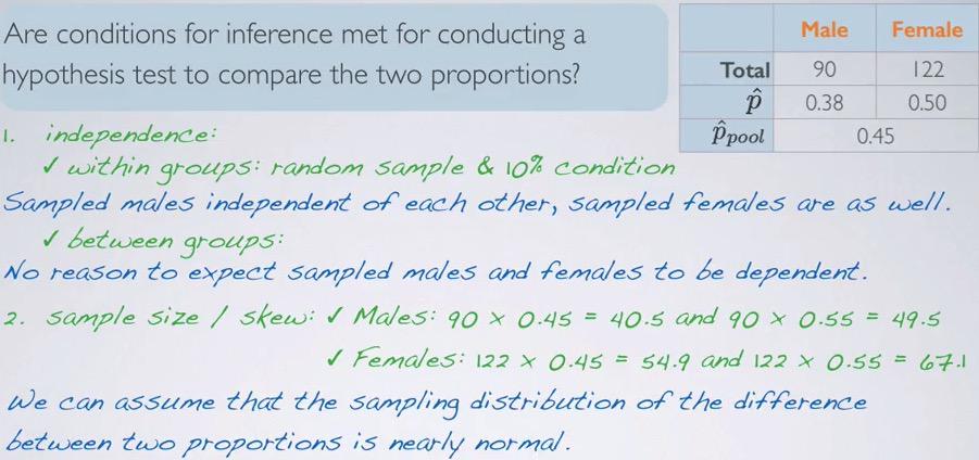
After we recalculate the p pool, we we check the conditions for hypothesis testing.

• Independence. Within groups, therer are less than 10% population for both female and male. Between groups, there are no dependent(paired) data, if it does paired, there should be at least equal number of female and male. Therefore we can conclude that sampled males are independent of each other, sampled females as well. We also expect that male and female are independent to one another.
• Sample size/skew. We calculate each of the sample size into our new p pool and validate the conditions of successes and failures for each female and male.If the quarduple value is at least 10, we can assume that sampling distribution of proportion differences is nearly normal.

Next, we proceed to calculate hypothesis testing.

Screenshot taken from Coursera 12:25

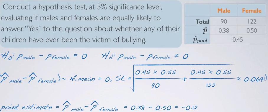
So you maybe notice something different. Yes, p-pool is not value that you use for null value! It only represent what value that represent equal proportion for both female and male. But since the p pool is equal for both male and female, the difference is still zero, hence the null value is zero. So calculating everything,

#1 = Male, 2 = Female

n_1 = 90
p_1 = 0.38

n_2 = 122
p_2 = 0.5

p_pool = 0.45
null = 0

SE = sqrt((p_pool*(1-p_pool)/n_1) + (p_pool*(1-p_pool)/n_2))
pe = p_1 - p_2

pnorm(pe,mean=null,sd=SE, lower.tail=pe < null) * 2

[1] 0.08257998

Based on the p-value and 5% significance level, we would failed to reject null hypothesis, and states there is no difference between males and females with respect to likelihood reporting their kids to being bullied

Summary

Calculating for standard error of two categorical variable, testing the difference, is different when we have confidence interval or hypothesis testing that have null value other than zero. We join standard error of both propotion of categorical variable. But for hypothesis testing that have null value zero, both of categorical variable proportion is not known. Hence we use pool proportion, joining successes divided by sample size of both categorical variables. The reason behind another discrepancy for hypothesis testing with null value zero, is that assumed that proportions are equal for levels in categorical variable, we have to use common proportions that fit both levels.

REFERENCES:

Dr. Mine Çetinkaya-Rundel, Cousera