Paired data and Bootstrapping
This will become the foundation for the inference for numerical variables. This blog will discuss how to compare mean for each of the group.Specifically how we can make inference other than CI(because median and other point estimate can't be fit in CLT). We also learn how to do bootstrapping (randomize permuation for each step), working for small example(less than 30, like t-distribution), and comparing many means (ANOVA).
Screenshot taken from Coursera 02:09
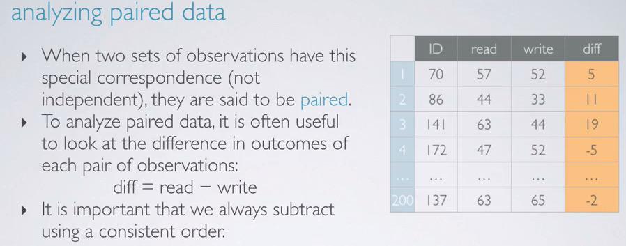
This is an examples where students' score being observed for their read and writing test. This have 200 data. This is of course read and writing are dependant variables. Students with high-achieving scores are most likely having both higher scores. This two variables is what we called paired data.
Parameter of Interest that we're going to observe is the population mean. But since we don't know the value, we're going to use average difference of sampled students as point estimate.
$$ PoI = \mu_\mathbf{diff}$$
$$ PO = \bar{x}_\mathbf{diff} $$
Screenshot taken from Coursera 03:36
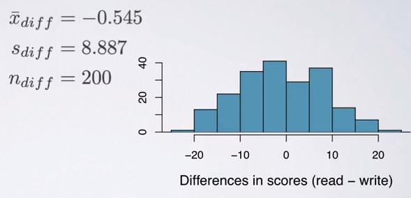
Here we have calculate each of the difference of the students and make a summary statistics. Now we should expect that the average difference is zero, but turn out it's not the exact value. Is the difference is due to chance? is it statiscally significant? To test this, we use previous tool, hypothesis testing.
Hypothesis Testing for Paired Data
Screenshot taken from Coursera 07:17
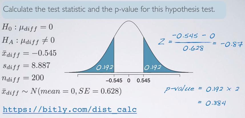
Now we can use Hypothesis Framework to test our data. The sample size is 200, which confirm higher than 30, but less than 10% population. The students is random sampled, so it is independent of one another. Than we can make a distribution, compute test statistics and shade the p-value. Standard Error can be get, we already have sample size and standard deviation. Because we investigate the different, we doubled the p-value.
This is what we can do in paired data, where data have 2 variables(can be more) but as long as it dependant, we can reduce to 1 variable. The null value is 0, but can be set with other value to your need. The benefits for HT paired data is same individuals: we can have pre/post studies about one person, identify the variable at the beginning and end of observation, we can have repeated measurement of groups. And when it's not about same individuals, we can use it on different(but dependant variables), such as twins, partners, family, etc.
CI intervals for Paired Data
Using the same examples earlier, we calculate its confidence interval. We don't want to just rejecting the hypothesis, but also measures its uncertainty. Recall that significance level used earlier is 5%, which equal to 95% confidence interval. Since we failed to reject null hypothesis, the observed outcome should be within the interval. The interval will be calculated as,
%load_ext rpy2.ipython
%%R

#95% = 1.96
#99% = 2.58

n = 200
mu = -0.545
s = 8.887
# z = 1.96
CL = 0.95
z = round(qnorm((1-CL)/2,lower.tail=F),digits=2)
SE = s/sqrt(n)
ME = z*SE


c(mu-ME,mu+ME)
Recall that the difference that we get is reading subtracted by writing, we can make a confident interval statement as, "We are 95% confident that high school students on average, reading is 1.78 lower to 0.69 higher than writing."
Comparing Independent Means
We already discussed earlier how we can compare two dependant variables, but how about independent? In this section we discuss how we can make hypothesis testing and confidence interval for independent variables.
Screenshot taken from Coursera 01:12
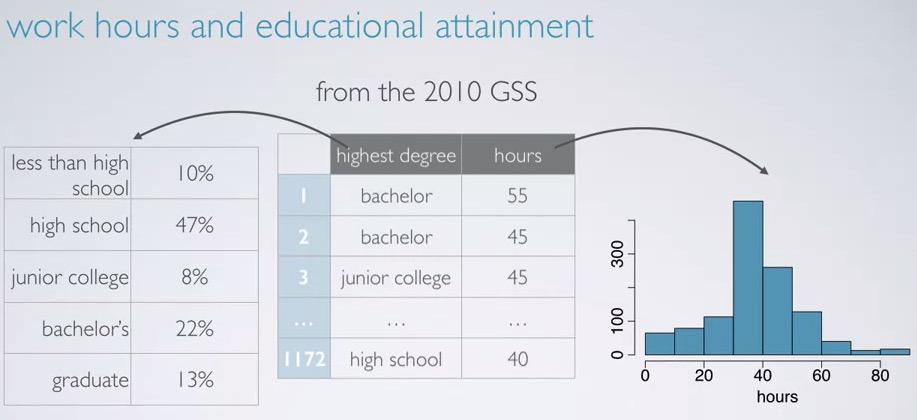
Let's take a look athe example of 2010 GSS, where among the variables are highest degree, categorical and hours, numerical discrete. We can used side-by-side boxplot to plot between categorical and numerical variables.But what we're currently concern about is whether they got college degree or not. This way we group the degrees into college degree and the opposite, no degree.
Screenshot taken from Coursera 04:20
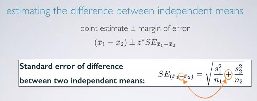
So to begin with, we use CI. As usual we estimate PoI and PE. our parameter interest this time, is the different between two variables, and point estimate is the difference in the sampled variables.
$$ PoI = \mu_\mathbf{col} - \mu_\mathbf{nocol}$$
$$ PO = \bar{x}_\mathbf{col} - \bar{x}_\mathbf{nocol} $$
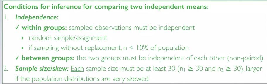
Next, we calculate the margin of error. Given the equation, we have our standard error. While explaining why the addition is beyond the scope of this blog, think about how the addition is a joint of two error variability of each of the variables. Therefore, the standard error will be higher.Because the calculations of standard error is different for independent vs dependent variables, we must validate the conditions. To be more precise, the requirements are:
Screenshot taken from Coursera 06:50
We see some similarities for confidence interval. In addition, pay attention to the groups. These groups must be independent. And the sample size must met the criteria. We already seen that the sample size is different for college vs no college, so we know that it can't be paired(different sample size, independent). We also see that both distributions are not very skewed and the sample size meet the criteria. If it dependent, we must revert back to paired CI earlier.
import numpy as np
Screenshot taken from Coursera 08:13
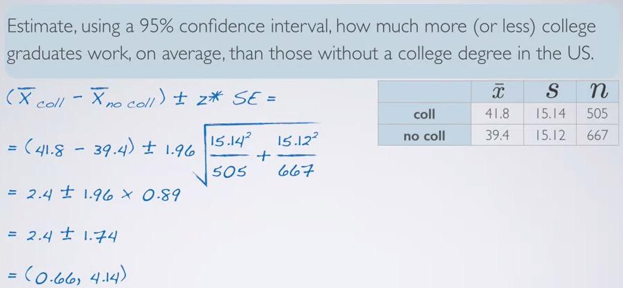
Then, after the data meet the criteria earlier, we can calculate CI based on the given parameters. What we get is positive 0.66 and 4.14. Since we know that CI is calculated based on $\bar{x}_\mathbf{coll} - \bar{x}_\mathbf{no coll}$, in CI statement, we say "College grads work on average is 0.66 to 4.14 hours more per week than those without a college degree.
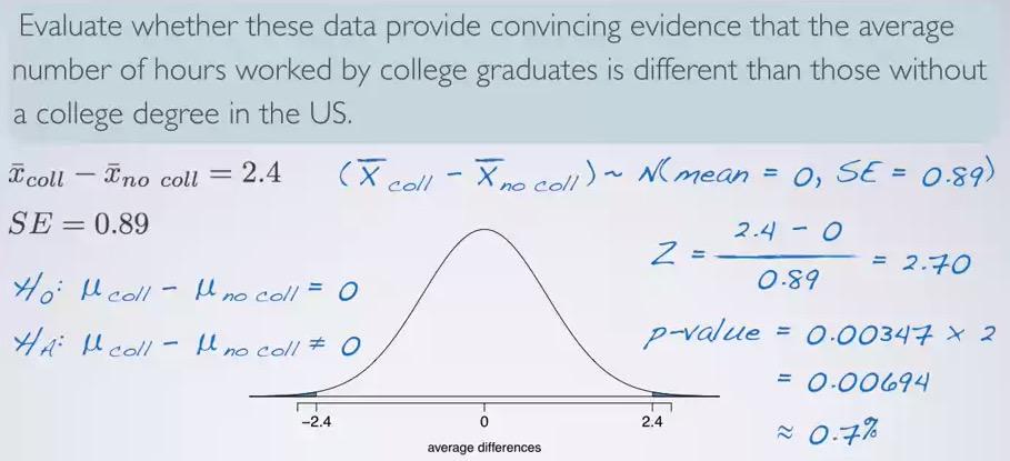
For hypothesis testing, we're being skeptical if there is no difference between college degree and without a degree. Alternative one can be different, less than, or greater than. Same conditions and SE have been meassured by CI earlier.
Screenshot taken from Coursera 13:08
%R pnorm(2.4,mean=0,sd=0.89,lower.tail=F)
%%R
s_1 = 3.4
s_2 = 2.7

n_1 = 18
n_2 = 18

sqrt(s_1**2/n_1 + s_2**2/n_2)
Calculating the p-value, what we get is 0.7%. Such small p-value would means that we reject the null hypothesis and favor the alternative. Interpret p-value for each of problem is often complex, the best way to interpret this is use the foundation definition of p-value, and work our way up the problem.
We know that null hypothesis is no difference of work hours on average between college degree and not college degree. We know the observe outcome, which is 2.4. We also know that more extreme, means that at least 2.4, and different means either direction. Based on that foundations, we can make HT statement,
"If there is no difference of work hours on average between college degree vs non college degree, there is 0.7% chance of obtaining random samples of 505 college and 667 non-college degree give average difference of work hours at least 2.4 hours". Readers can conclude, that such small probability is very rare, and won't likely happen due to chance.Beside the p-value definition, we also have to mention each of the sample size. Because different sample size would yield different outcome, hence different p-value.
Bootstrapping
Screenshot taken from Coursera 01:35
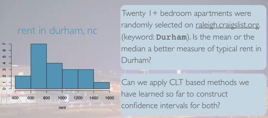
So we have twenty samples and skewed distribution. This data is taken from search engine of raleigh, on apartment in Durham, city where Duke university is located. Because this is skewed data, median is better fit. We can't use CLT, since we calculate the median, and the sample size is less than 30. Since no known tools that we can used so far,introduced Bootstrapping.Bootstrapping is different from sampling distribution in that bootstrapping generate samples from sample with replacement, sampling distribution generate samples from population with replacement.
Screenshot taken from Coursera 03:46
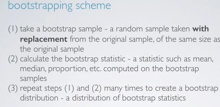
This is what we have to do in bootstrapping. The idea is, there might be some similar value within the population. So we're taking random sampling with replacement, from values in sample. So it's like taking with replacement sampling of Bootstrap from the sample, and bootstrap consider the sample as the population. By doing this, we're regenerate fake data from the samples. Doing this of course we have to have independent variables. Bootstrap can use median,proportion, or any other point estimate.Take a look here where we have only have 5 samples, but resampling with replacement with 6 bootstrap.
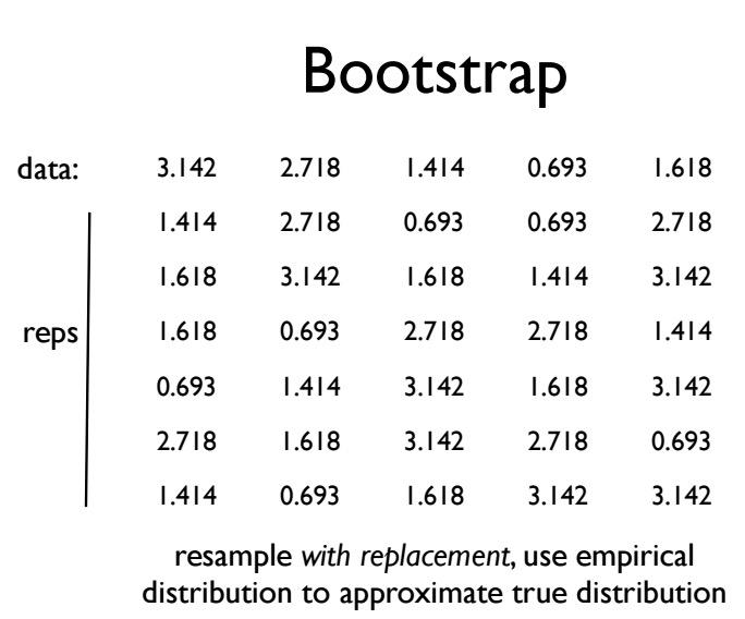
Screenshot taken from CS109Harvard
Then bootstrap will perform same step like sampling distribution, but this time its different, and called a distribution of bootstrap statistics. This is very useful method. Even Harvard statistics professor,Joe Blitztein in the CS109 Harvard 2013 Data Science online class, stated, and I quoted here, " Bootstrap is one of the biggest statistical breakthrough in the 21th century".
Screenshot taken from Coursera 05:50
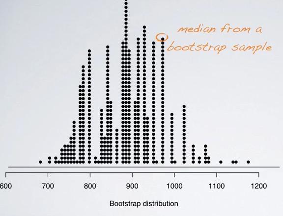
So based on such small sample size, we can construct bootstrap distribution. this should give us a sense of median from the population distribution. If you're taking $676 apartment from bootstrap, it's likely that you also have similar value within the population. So next, how do construct CI based on bootstrap statistics?
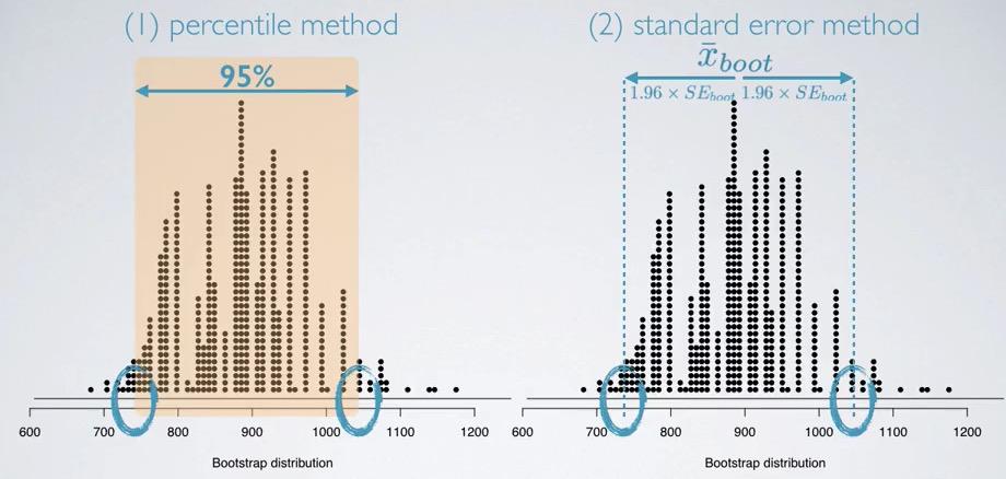
Screenshot taken from Coursera 07:17
First we can use percentile method, the bootstrap distribution can be considered as centered around the population median.Because this looks like normal distribution, we can estimate 95% interval and assign lower bound and upper bound.
Using standard error method, we can calculate the Standard error, and assigning the point estimate, creating upper bound and lower bound. We don't have to use CLT, but we may take extra steps for regenerating bootstrap sample, using computation.
Consider the following examples.
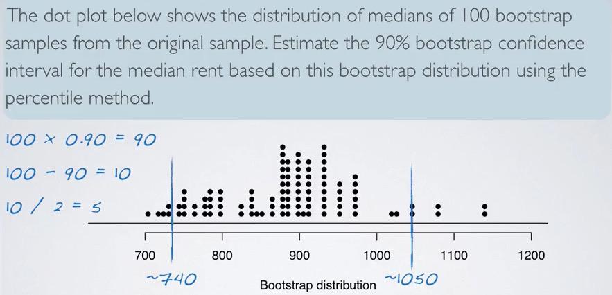
Screenshot taken from Coursera 08:54
Using the percentiles method, we simulated the distribution and cut off 5 dot points on each side. Recall that the dot plot is the median of one bootstrap sample. Doing bootstrap doesn't mean we can't infer the population parameter, CI is still always about the population. So we can say, "We are 95% confident that median rent of 1+ apartments in Durham is somwhere between 740 and 1050 dollar.
Screenshot taken from Coursera 11:02
From the bootstrap simulation, we're given mean and SE. Using that as a basis, we calculate the interval
%%R

#95% = 1.96
#99% = 2.58

n = 100
mu = 882.515
# s = 89.5758
# z = 1.96
CL = 0.9
z = round(qnorm((1-CL)/2,lower.tail=F),digits=2)
# SE = s/sqrt(n)
SE = 89.5759
ME = z*SE


c(mu-ME,mu+ME)
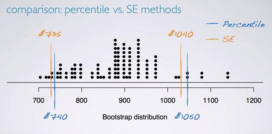
In the plot above, we see that the intervals are different, but pretty close.
Bootstrap Limitation
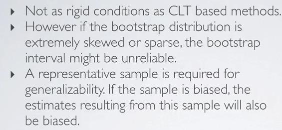
Screenshot taken from Coursera 12:14
Bootstrap vs Sampling distribution
- samping distritbuion with replacement from population, where bootsrap with replacement from sample
- Both are distributions of sample statistics. CLT can explicitly describe the distribution of the population, where bootstrap also describe that using one sample.
Summary
Bootstrap can be created by using with replacement in one sample. This is different from sampling distribution, where it takes with replacement from population.We can use percentile method; take 100 sample size bootstrap and cut off the sided for XX% interval, or calculate percentile based on the known condition that the distribution is normal, use point estimate bootstrap and standard error bootstrap.There's one weakness of bootstrap, is that when you have skew and sparse bootstrap distribution, it's not reliable.
Paired data, is when you have one observation dependent on other variable.We can use these set differences as a basis to use hypothesis testing and confidence interval.