Feature Selection with scikit-learn
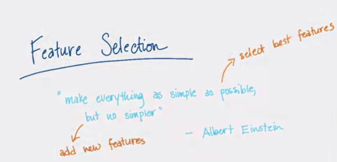
Feature Selection is one of thing that we should pay attention when building machine learning algorithm. For all features available, there might be some unnecessary features that will overfitting your predictive model if you include it. So choose best features that's going to have good perfomance, and prioritize that. On the other hand, we may don't see that some features, that we really need is missing (in the case of using EDA). What we want to do is synthesize a new feature based on features available.
A new Enron Feature
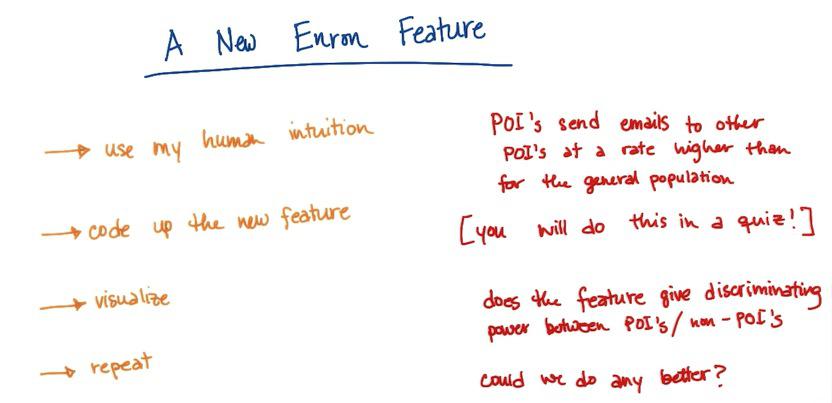
Let's take a look at the enron dataset. For those who doesn't know about Enron dataset, read my earlier post. Create a new feature, based on the Enron dataset, is as follows:
- Use your human intuition. Ask a question about the dataset that you have. Then if the feature for the answer that you asked is not available, try if you can synthesize based on existing features.For example, POI (person of interest) send email with other POI at higher rate than general population.
- Code up the new feature. If you have choose by intuition what could be happening that your features can't explaining, then you can create by code it.
- Visualize. See if you can understand what's this data all about. if you synthesized it, did you get the information as expected?
- Repeat the process. Try to synthesize from other features and see if you can get best features out of it.
%%writefile poi_flag_email.py

#!/usr/bin/python

###
### in poiFlagEmail() below, write code that returns a boolean
### indicating if a given emails is from a POI
###

import sys
import reader
import poi_emails

def getToFromStrings(f):
    f.seek(0)
    to_string, from_string, cc_string   = reader.getAddresses(f)
    to_emails   = reader.parseAddresses( to_string )
    from_emails = reader.parseAddresses( from_string )
    cc_emails   = reader.parseAddresses( cc_string )

    return to_emails, from_emails, cc_emails


### POI flag an email

def poiFlagEmail(f):
    """ given an email file f,
        return a trio of booleans for whether that email is
        to, from, or cc'ing a poi """

    to_emails, from_emails, cc_emails = getToFromStrings(f)

    ### list of email addresses of all the POIs
    poi_email_list = poi_emails.poiEmails()

    to_poi = False
    from_poi = False
    cc_poi   = False

    ### to_poi and cc_poi are related functions, which flag whether
    ### the email under inspection is addressed to a POI, or if a POI is in cc
    ### you don't have to change this code at all

    ### there can be many "to" emails, but only one "from", so the
    ### "to" processing needs to be a little more complicated
    if to_emails:
        ctr = 0
        while not to_poi and ctr < len(to_emails):
            if to_emails[ctr] in poi_email_list:
                to_poi = True
            ctr += 1
    if cc_emails:
        ctr = 0
        while not to_poi and ctr < len(cc_emails):
            if cc_emails[ctr] in poi_email_list:
                cc_poi = True
            ctr += 1


    #################################
    ######## your code below ########
    ### set from_poi to True if #####
    ### the email is from a POI #####
    #################################


    if from_emails and from_emails[0] in poi_email_list:
        from_poi = True


    #################################
    return to_poi, from_poi, cc_poi
# %%writefile new_enron_feature.py

#!/usr/bin/python

import os
import sys
import zipfile
from poi_flag_email import poiFlagEmail, getToFromStrings

data_dict = {}

with zipfile.ZipFile('emails.zip', "r") as z:
    z.extractall()

for email_message in os.listdir("emails"):
    if email_message == ".DS_Store":
        continue
    message = open(os.getcwd()+"/emails/"+email_message, "r")
    to_addresses, from_addresses, cc_addresses = getToFromStrings(message)

    to_poi, from_poi, cc_poi = poiFlagEmail(message)

    for recipient in to_addresses:
        if recipient not in data_dict:
            data_dict[recipient] = {"from_poi_to_this_person":0}
        else:
            if from_poi:
                data_dict[recipient]["from_poi_to_this_person"] += 1

    message.close()

for item in data_dict:
    print item, data_dict[item]

#######################################################
def submitData():
    return data_dict
%%writefile visualize_new_feature.py

import pickle
from get_data import getData

def computeFraction( poi_messages, all_messages ):
    """ given a number messages to/from POI (numerator)
        and number of all messages to/from a person (denominator),
        return the fraction of messages to/from that person
        that are from/to a POI
   """


    ### you fill in this code, so that it returns either
    ###     the fraction of all messages to this person that come from POIs
    ###     or
    ###     the fraction of all messages from this person that are sent to POIs
    ### the same code can be used to compute either quantity

    ### beware of "NaN" when there is no known email address (and so
    ### no filled email features), and integer division!
    ### in case of poi_messages or all_messages having "NaN" value, return 0.
    fraction = 0.
    if all_messages == 'NaN':
        return fraction

    if poi_messages == 'NaN':
        poi_messages = 0

    fraction = float(poi_messages)/float(all_messages)

    return fraction


data_dict = getData()

submit_dict = {}
for name in data_dict:

    data_point = data_dict[name]

    print
    from_poi_to_this_person = data_point["from_poi_to_this_person"]
    to_messages = data_point["to_messages"]
    fraction_from_poi = computeFraction( from_poi_to_this_person, to_messages )
    print fraction_from_poi
    data_point["fraction_from_poi"] = fraction_from_poi


    from_this_person_to_poi = data_point["from_this_person_to_poi"]
    from_messages = data_point["to_messages"]
    fraction_to_poi = computeFraction( from_this_person_to_poi, from_messages )
    print fraction_to_poi
    submit_dict[name]={"from_poi_to_this_person":fraction_from_poi,
                       "from_this_person_to_poi":fraction_to_poi}
    data_point["fraction_to_poi"] = fraction_to_poi


#####################

def submitDict():
    return submit_dict
Beware of Bugs
Let's hear Katie and the team when facing bug in Enron dataset.
When Katie was working on the Enron POI identifier, she engineered a feature that identified when a given person was on the same email as a POI. So for example, if Ken Lay and Katie Malone are both recipients of the same email message, then Katie Malone should have her "shared receipt" feature incremented. If she shares lots of emails with POIs, maybe she's a POI herself.
Here's the problem: there was a subtle bug, that Ken Lay's "shared receipt" counter would also be incremented when this happens. And of course, then Ken Lay always shares receipt with a POI, because he is a POI. So the "shared receipt" feature became extremely powerful in finding POIs, because it effectively was encoding the label for each person as a feature.
We found this first by being suspicious of a classifier that was always returning 100% accuracy. Then we removed features one at a time, and found that this feature was driving all the performance. Then, digging back through the feature code, we found the bug outlined above. We changed the code so that a person's "shared receipt" feature was only incremented if there was a different POI who received the email, reran the code, and tried again. The accuracy dropped to a more reasonable level.
We take a couple of lessons from this:
- Anyone can make mistakes--be skeptical of your results!
- 100% accuracy should generally make you suspicious. Extraordinary claims require extraordinary proof.
- If there's a feature that tracks your labels a little too closely, it's very likely a bug!
- If you're sure it's not a bug, you probably don't need machine learning--you can just use that feature alone to assign labels.
Getting Rid of Features
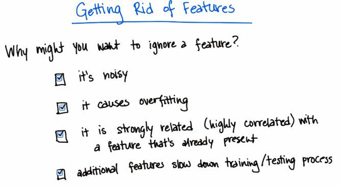
- Noisy. Every features have their own noise. So to ignore feature can have less noisy.
- Overfitting. We already talked about this, It will overfit the data, because the model with unnecessary feature include. The feature that might not be important, or redundant, or not increase the performance our model.
- This could be feature where for example distance, return two feature (maybe the people gathering the data is different) which is cm and feet. This is the same, and could potentially break your algorithm in mathematical process. Either delete one of them, or maybe create new feature, join them to one feature and exclude both.
- Slow down your training process. We may want to reduce our feature so it doesn't take days or maybe years at worst.
Features vs Information
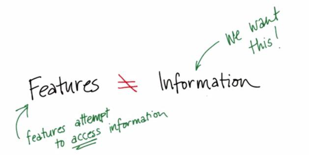
Features is not the same thing as Information. Is not technically that if you have a lot of features, then you would have gained much information. What do we want is Information. And if minimum amount of features would give you enough information, then you should do that. It's like quantity vs quality. compare to have many quantity(features), you only want to pick those with quality(information)
Univariate Feature Selection
And here I'm repeating what Instructor at Udacity stated:
There are several go-to methods of automatically selecting your features in sklearn. Many of them fall under the umbrella of univariate feature selection, which treats each feature independently and asks how much power it gives you in classifying or regressing.
There are two big univariate feature selection tools in sklearn: SelectPercentile and SelectKBest. The difference is pretty apparent by the names: SelectPercentile selects the X% of features that are most powerful (where X is a parameter) and SelectKBest selects the K features that are most powerful (where K is a parameter).
A clear candidate for feature reduction is text learning, since the data has such high dimension. We actually did feature selection in the Sara/Chris email classification problem during the first few mini-projects; you can see it in the code in tools/email_preprocess.py .
Let's take a look at the selectpercentile at sklearn
class sklearn.feature_selection.SelectPercentile(score_func=<function f_classif at 0x34fca28>, percentile=10)score_func = you could take f_classif module from sklearn.feature_selection
percentile = what percentage of features you want to select. Here sklearn only take top 10% features that contain the most information
In text learning you can also filter the most frequent word. Take a look at this sklearn tfidfVectorizer, that I use earlier in my blog post.
vectorizer = TFidfVectorizer(sublinear_tf=True,max_df=0.5,stop_words='english')the vectorizer will then take off words that in 50% of the document, besides stop_words. The idea behind this is that if the words are so common, it may not be the feature that distinct each of the document. In other word, not have much information. You can also combine this with do SelectPercentile after you have done the vectorizer.
Bias vs Variance
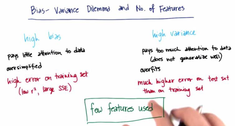
You know that high bias is when your perfomance low on training set(you can test it by residual error or sum of squared error). In terms of number of features you may select too few features in your model.
As also for high variance, you're too committed to the data, resulting to act poorly on the test set. This also means that you have too much features in your model. Be careful as you don't also try all the features to try to minimize SSE in your training dataset.
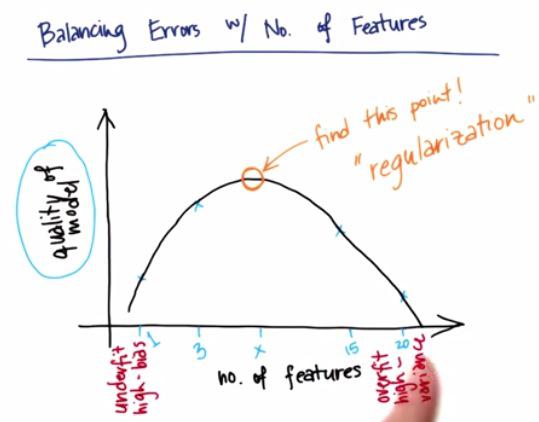
Suppose that you tried number of features and check the quality of your model. Then as you test it, you're getting more fit of your data, thus overfitting and the quality reduced. What we want to do is at the peak of the curve as graph above.
The important thing to take away is, if you have score your performance in training set poorly, then you have high bias in your learning model. On the other hand if you have great performance on your training set, but fail when you use it in a test set, then there's a strong indication that you have high variance. You can test how much features you need by keeping this in mind, and achieve large r^2 with low SSE.
Regularization
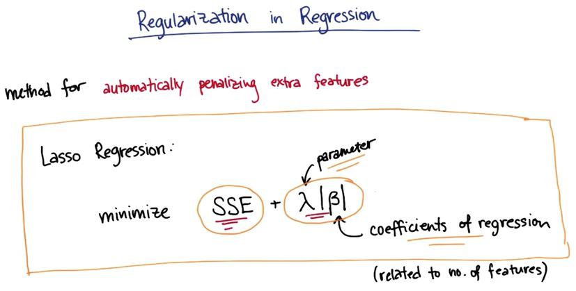
There's also method called regurization, which takes penalty as we gain more features. The higher the lambda, the more strength it will penalize the features. This is other smart moves other than feature selection.
Suppose we want to minimize SSE of our model. In doing so, we gather as much features available to us to minimize the SSE. Adding regularization will penalize our model as we get more features, therefore automatically handle tradeoff between low SSE and many features, vs high SSE and low features. Therefore the features that's not important will take higher penalty, and the features with most information will have lower penalty.
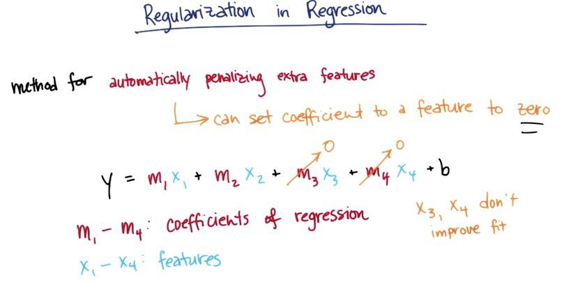
We see that regularization act as coefficient for the features. When the features not gain any performance in our model, the regularization coeffecient will set to zero, therefore nullfying x3 and x4, which then left x1 and x2.
Keep in mind when setting the regularization value(lambda). Too high and it will penalize your data too much(underfit), too low and it will penalize poorly resulting in overfitting. You may want to step your lambda value in repeating process.
This is code snippet from sklearn documentation about lasso
from sklearn.linear_model import Lasso
features,labels = getMyData()
regression = Lasso
regression.fit(features,labels)
regression.predict([[2,4]])
print regression.coef_#This will give you coeffecients of regression of each of your feature
For more information on mathematical process behind regularization on linear regression, logistic regression, and how it tackles overfitting, please head over my other blog posts.
Mini Project
As usual, because this blog post are the note that I have taken from Udacity course, Here I attack some of the problem they have at their mini project. You can see the link of the course for this note at the bottom of this page.
Katie explained in a video a problem that arose in preparing Chris and Sara’s email for the author identification project; it had to do with a feature that was a little too powerful (effectively acting like a signature, which gives an arguably unfair advantage to an algorithm). You’ll work through that discovery process here.
This bug was found when Katie was trying to make an overfit decision tree to use as an example in the decision tree mini-project. A decision tree is classically an algorithm that can be easy to overfit; one of the easiest ways to get an overfit decision tree is to use a small training set and lots of features. If a decision tree is overfit, would you expect the accuracy on a test set to be very high or pretty low?
The accuracy would be very high on the training set, but would plummet once it was actually tested.
A classic way to overfit an algorithm is by using lots of features and not a lot of training data. You can find the starter code in feature_selection/find_signature.py. Get a decision tree up and training on the training data, and print out the accuracy. How many training points are there, according to the starter code?
%load find_signature.py
%%writefile find_signature.py
import pickle
import numpy
numpy.random.seed(42)


### the words (features) and authors (labels), already largely processed
words_file = "../text_learning/your_word_data.pkl" ### you made this in previous mini-project
authors_file = "../text_learning/your_email_authors.pkl"  ### this too
word_data = pickle.load( open(words_file, "r"))
authors = pickle.load( open(authors_file, "r") )


### test_size is the percentage of events assigned to the test set (remainder go into training)
from sklearn import cross_validation
features_train, features_test, labels_train, labels_test = cross_validation.train_test_split(word_data, authors, test_size=0.1, random_state=42)


from sklearn.feature_extraction.text import TfidfVectorizer
vectorizer = TfidfVectorizer(sublinear_tf=True, max_df=0.5,
                             stop_words='english')
features_train = vectorizer.fit_transform(features_train).toarray()
features_test  = vectorizer.transform(features_test).toarray()


### a classic way to overfit is to use a small number
### of data points and a large number of features
### train on only 150 events to put ourselves in this regime
features_train = features_train[:150]
labels_train   = labels_train[:150]
What’s the accuracy of the decision tree you just made? (Remember, we're setting it up to be overfit--this number should be relatively low.)
from sklearn.tree import DecisionTreeClassifier
clf = DecisionTreeClassifier()
clf.fit(features_train,labels_train)
clf.score(features_test,labels_test)
Yes, it has an accuracy much higher than it should be.
Take your (overfit) decision tree and use the featureimportances attribute to get a list of the relative importance of all the features being used. We suggest iterating through this list (it’s long, since this is text data) and only printing out the feature importance if it’s above some threshold (say, 0.2--remember, if all words were equally important, each one would give an importance of far less than 0.01). What’s the importance of the most important feature? What is the number of this feature?
importances = clf.feature_importances_
import numpy as np
indices = np.argsort(importances)[::-1]
print 'Feature Ranking: '
for i in range(10):
    print "{} feature no.{} ({})".format(i+1,indices[i],importances[indices[i]])
In order to figure out what words are causing the problem, you need to go back to the TfIdf and use the feature numbers (you got those in Part 2) to get the associated words. You can return a list of all the words in the TfIdf by calling get_feature_names() on it; pull out the word that’s causing most of the discrimination of the decision tree. What is it? Does it make sense as a word that’s uniquely tied to either Chris Germany or Sara Shackleton, a signature of sorts?
vectorizer.get_feature_names()[33614]
This word seems like an outlier in a certain sense, so let’s remove it and refit. Go back to text_learning/vectorize_text.py, and remove this word from the emails using the same method you used to remove “sara”, “chris”, etc. Rerun vectorize_text.py, and once that finishes, rerun find_signature.py. Any other outliers pop up? What word is it? Seem like a signature-type word? (Define an outlier as a feature with importance >0.2, as before).
%load find_signature.py
import pickle
import numpy
numpy.random.seed(42)


### the words (features) and authors (labels), already largely processed
words_file = "../text_learning/your_word_data.pkl" ### you made this in previous mini-project
authors_file = "../text_learning/your_email_authors.pkl"  ### this too
word_data = pickle.load( open(words_file, "r"))
authors = pickle.load( open(authors_file, "r") )


### test_size is the percentage of events assigned to the test set (remainder go into training)
from sklearn import cross_validation
features_train, features_test, labels_train, labels_test = cross_validation.train_test_split(word_data, authors, test_size=0.1, random_state=42)


from sklearn.feature_extraction.text import TfidfVectorizer
vectorizer = TfidfVectorizer(sublinear_tf=True, max_df=0.5,
                             stop_words='english')
features_train = vectorizer.fit_transform(features_train).toarray()
features_test  = vectorizer.transform(features_test).toarray()


### a classic way to overfit is to use a small number
### of data points and a large number of features
### train on only 150 events to put ourselves in this regime
features_train = features_train[:150]
labels_train   = labels_train[:150]
from sklearn.tree import DecisionTreeClassifier
clf = DecisionTreeClassifier()
clf.fit(features_train,labels_train)
clf.score(features_test,labels_test)
importances = clf.feature_importances_
import numpy as np
indices = np.argsort(importances)[::-1]
print 'Feature Ranking: '
for i in range(10):
    print "{} feature no.{} ({})".format(i+1,indices[i],importances[indices[i]])
vectorizer.get_feature_names()[14343]
Update vectorize_test.py one more time, and rerun. Then run find_signature.py again. Any other important features (importance>0.2) arise? How many? Do any of them look like “signature words”, or are they more “email content” words, that look like they legitimately come from the text of the messages?
import pickle
import numpy
numpy.random.seed(42)


### the words (features) and authors (labels), already largely processed
words_file = "../text_learning/your_word_data.pkl" ### you made this in previous mini-project
authors_file = "../text_learning/your_email_authors.pkl"  ### this too
word_data = pickle.load( open(words_file, "r"))
authors = pickle.load( open(authors_file, "r") )


### test_size is the percentage of events assigned to the test set (remainder go into training)
from sklearn import cross_validation
features_train, features_test, labels_train, labels_test = cross_validation.train_test_split(word_data, authors, test_size=0.1, random_state=42)


from sklearn.feature_extraction.text import TfidfVectorizer
vectorizer = TfidfVectorizer(sublinear_tf=True, max_df=0.5,
                             stop_words='english')
features_train = vectorizer.fit_transform(features_train).toarray()
features_test  = vectorizer.transform(features_test).toarray()


### a classic way to overfit is to use a small number
### of data points and a large number of features
### train on only 150 events to put ourselves in this regime
features_train = features_train[:150]
labels_train   = labels_train[:150]
from sklearn.tree import DecisionTreeClassifier
clf = DecisionTreeClassifier()
clf.fit(features_train,labels_train)
clf.score(features_test,labels_test)
importances = clf.feature_importances_
import numpy as np
indices = np.argsort(importances)[::-1]
print 'Feature Ranking: '
for i in range(10):
    print "{} feature no.{} ({})".format(i+1,indices[i],importances[indices[i]])
vectorizer.get_feature_names()[21323]
Yes, there is one more word ("houectect"). Your guess about what this word means is as good as ours, but it doesn't look like an obvious signature word so let's keep moving.
What’s the accuracy of the decision tree now? Remember, the whole point was to see if we could get it to overfit--a sensible result is one where the accuracy isn't that great!
clf.score(features_test,labels_test)
