PCA with scikit-learn
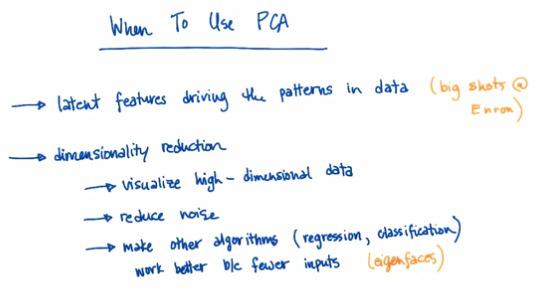
PCA is used thoroughly for most of the time in visualization data, alongside feature set compression. It's hard (othwerwise impossible) to interpret the data with more than three dimension. So we reduce it to two/third dimension, allow us to make the visualization. This could come very handy if we want to capture the general information about the data, or to present it as business context. But it's not the tool that we use for combining two features, or compress it, as PCA throws some (important) information.
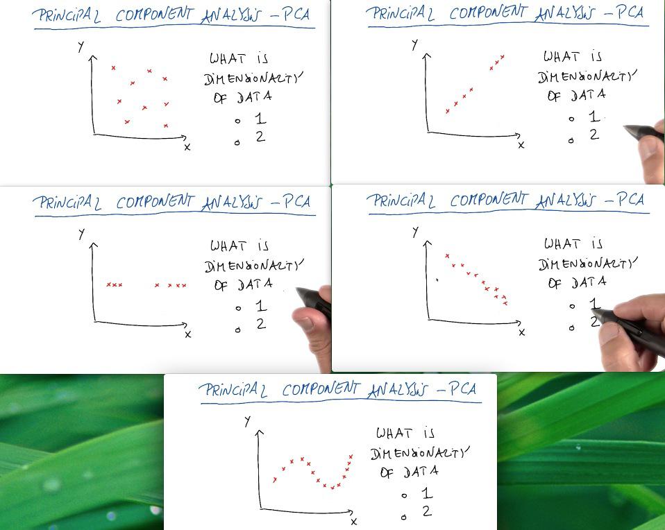
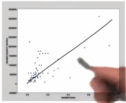
For the first case the data is well distributed among 2d graph. For the two and third case, the data is actually drawn for 1 line graph, and we can say that it's actually still one dimension. The third graph, while it's true for 2d, but we can still capture the trends of the data by drawing straight line, and treat deviation as noise. The last graph is what we can consider as 2D graph. It may has definite curve, but we can only draw straight line to reduce the dimension using PCA.
For more information about the fundamentals of mathematical process behind PCA, what to do, and advice please visit my other blog posts.
How PCA works
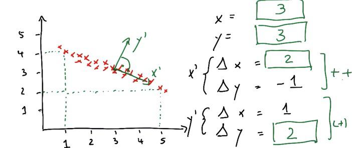
PCA works as these simple steps. Assign new x prime in horizontal line (trends of the data), and put the orthogonal as the ones that have less noise.
These new data center have it's own average weight. We can see the underlying center point has an x prime(delta x/y) and y prime(delta x/y). These will be the fundamentals of location in reduced dimension later.
All data in the graph is PCA-ready.The PCA also treats asymmetrical lines, which doesn't care input/output (third graph in this particular), vertical/horizontal, the PCA doesn't entail 1D graph to reduce the dimension. Well I say, that's pretty cool! Haha :)
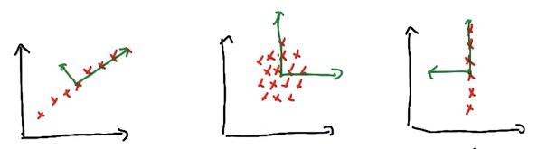
And for which of major axis dominates, we know that from seeing the graph first and third, it's a clear winner, which eigenvalues are bigger from another. The first graph have x with bigger eigenvalue than y, the orthogonal, which has zero. And so for the third graph. Interesting enough, the graph in the middle have same eigenvalues, same magnitude which gives no clear major axis.
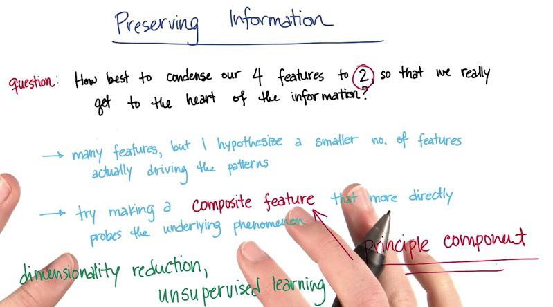
Suppose you have 4 features (square ft, number of rooms, school ranking, and the safety problems) to predict the price of a house. Considering maybe you want to have visualization of 2 dimension, you truncate all features to 2 dimension, size and neighborhood. If you don't know any number of features and only want to take n features, you want to choose SelectKBest from sklearn, or SelectPercentile to have n-percentage from features.
After that you want to create these composite feature, as your machine learning feature. This is what PCA means.
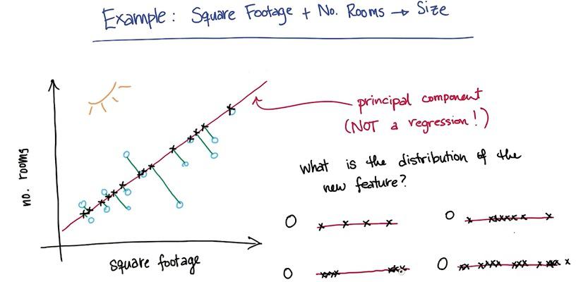
This is the difference between PCA and regression (you may want to check this post. In PCA, you take the perpendicular of a point projected to the line. This is why PCA may not be used to hone the regression. It only used to make visualization and get better insights.
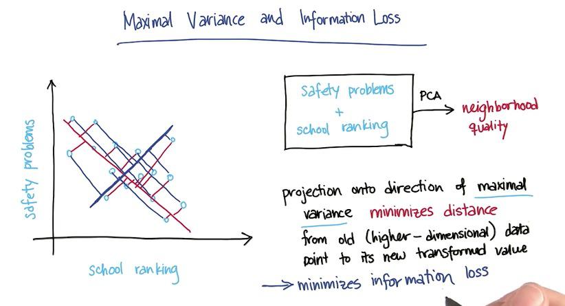
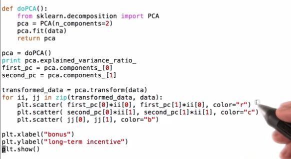
In this example we have "safety problems" and "school ranking" that we want to latent one feature in the data, maybe "neighborhood.The PCA must be choosing whichever direction of a projection line that retain most of the information as it can. Here PCA chose red one over the blue line, because the red one minimize sum of error over all data points. With this projection, we have retains much of information as we can.
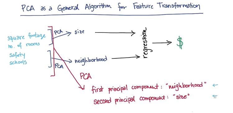
Here the PCA works as unsupervised learning algorithm. For perhaps infinite number of features, it cluster the category of those features. Here's PCA cluster 4 features to 2 features, size and neighborhood. As it caught 2 trends among all these features. It makes as a regression to predict the housing prices.
PCA on Enron Finance Data
Mini Project
As usual, because this blog post are the note that I have taken from Udacity course, you can see the link of the course for this note at the bottom of the page. Here I attack some of the problem they have at their mini project.
Our discussion of PCA spent a lot of time on theoretical issues, so in this mini-project we’ll ask you to play around with some sklearn code. The eigenfaces code is interesting and rich enough to serve as the testbed for this entire mini-project.
The starter code can be found in pca/eigenfaces.py. This was mostly taken from the example found here, on the sklearn documentation.
%load eigenfaces.py
%pylab inline
# %%writefile eigenfaces.py

"""
===================================================
Faces recognition example using eigenfaces and SVMs
===================================================

The dataset used in this example is a preprocessed excerpt of the
"Labeled Faces in the Wild", aka LFW_:

  http://vis-www.cs.umass.edu/lfw/lfw-funneled.tgz (233MB)

  .. _LFW: http://vis-www.cs.umass.edu/lfw/

  original source: http://scikit-learn.org/stable/auto_examples/applications/face_recognition.html

"""


print __doc__

from time import time
import logging
import pylab as pl
import numpy as np

from sklearn.cross_validation import train_test_split
from sklearn.datasets import fetch_lfw_people
from sklearn.grid_search import GridSearchCV
from sklearn.metrics import classification_report
from sklearn.metrics import confusion_matrix
from sklearn.decomposition import RandomizedPCA
from sklearn.svm import SVC

# Display progress logs on stdout
logging.basicConfig(level=logging.INFO, format='%(asctime)s %(message)s')


###############################################################################
# Download the data, if not already on disk and load it as numpy arrays

lfw_people = fetch_lfw_people(min_faces_per_person=70, resize=0.4)

# introspect the images arrays to find the shapes (for plotting)
n_samples, h, w = lfw_people.images.shape
np.random.seed(42)

# fot machine learning we use the 2 data directly (as relative pixel
# positions info is ignored by this model)
X = lfw_people.data
n_features = X.shape[1]

# the label to predict is the id of the person
y = lfw_people.target
target_names = lfw_people.target_names
n_classes = target_names.shape[0]

print "Total dataset size:"
print "n_samples: %d" % n_samples
print "n_features: %d" % n_features
print "n_classes: %d" % n_classes


###############################################################################
# Split into a training set and a test set using a stratified k fold

# split into a training and testing set
X_train, X_test, y_train, y_test = train_test_split(X, y, test_size=0.25, random_state=42)


def pcaTrainAndPredict(n_components):
    ###############################################################################
    # Compute a PCA (eigenfaces) on the face dataset (treated as unlabeled
    # dataset): unsupervised feature extraction / dimensionality reduction
#     n_components = 150

    print "Extracting the top %d eigenfaces from %d faces" % (n_components, X_train.shape[0])
    t0 = time()
    pca = RandomizedPCA(n_components=n_components, whiten=True).fit(X_train)
    print "done in %0.3fs" % (time() - t0)

    eigenfaces = pca.components_.reshape((n_components, h, w))

    print "Projecting the input data on the eigenfaces orthonormal basis"
    t0 = time()
    X_train_pca = pca.transform(X_train)
    X_test_pca = pca.transform(X_test)
    print "done in %0.3fs" % (time() - t0)


    ###############################################################################
    # Train a SVM classification model

    print "Fitting the classifier to the training set"
    t0 = time()
    param_grid = {
             'C': [1e3, 5e3, 1e4, 5e4, 1e5],
              'gamma': [0.0001, 0.0005, 0.001, 0.005, 0.01, 0.1],
              }
    clf = GridSearchCV(SVC(kernel='rbf', class_weight='auto'), param_grid)
    clf = clf.fit(X_train_pca, y_train)
    print "done in %0.3fs" % (time() - t0)
    print "Best estimator found by grid search:"
    print clf.best_estimator_


    ###############################################################################
    # Quantitative evaluation of the model quality on the test set

    print "Predicting the people names on the testing set"
    t0 = time()
    y_pred = clf.predict(X_test_pca)
    print "done in %0.3fs" % (time() - t0)

    print classification_report(y_test, y_pred, target_names=target_names)
    print confusion_matrix(y_test, y_pred, labels=range(n_classes))


pcaTrainAndPredict(150)
###############################################################################
# Qualitative evaluation of the predictions using matplotlib

def plot_gallery(images, titles, h, w, n_row=3, n_col=4):
    """Helper function to plot a gallery of portraits"""
    pl.figure(figsize=(1.8 * n_col, 2.4 * n_row))
    pl.subplots_adjust(bottom=0, left=.01, right=.99, top=.90, hspace=.35)
    for i in range(n_row * n_col):
        pl.subplot(n_row, n_col, i + 1)
        pl.imshow(images[i].reshape((h, w)), cmap=pl.cm.gray)
        pl.title(titles[i], size=12)
        pl.xticks(())
        pl.yticks(())


# plot the result of the prediction on a portion of the test set

def title(y_pred, y_test, target_names, i):
    pred_name = target_names[y_pred[i]].rsplit(' ', 1)[-1]
    true_name = target_names[y_test[i]].rsplit(' ', 1)[-1]
    return 'predicted: %s\ntrue:      %s' % (pred_name, true_name)

prediction_titles = [title(y_pred, y_test, target_names, i)
                         for i in range(y_pred.shape[0])]

plot_gallery(X_test, prediction_titles, h, w)

# plot the gallery of the most significative eigenfaces

eigenface_titles = ["eigenface %d" % i for i in range(eigenfaces.shape[0])]
plot_gallery(eigenfaces, eigenface_titles, h, w)

pl.show()


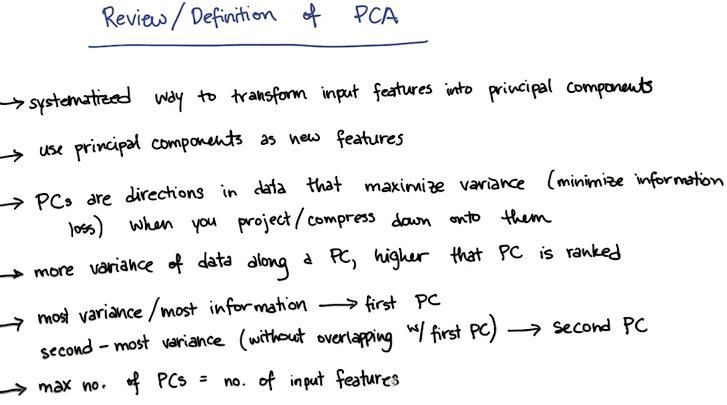
We mentioned that PCA will order the principal components, with the first PC giving the direction of maximal variance, second PC has second-largest variance, and so on. How much of the variance is explained by the first principal component? The second?
pca.explained_variance_ratio_[:2]
Now you'll experiment with keeping different numbers of principal components. In a multiclass classification problem like this one (more than 2 labels to apply), accuracy is a less-intuitive metric than in the 2-class case. Instead, a popular metric is the F1 score.
We’ll learn about the F1 score properly in the lesson on evaluation metrics, but you’ll figure out for yourself whether a good classifier is characterized by a high or low F1 score. You’ll do this by varying the number of principal components and watching how the F1 score changes in response.
As you add more principal components as features for training your classifier, do you expect it to get better or worse performance?
Better
Change n_components to the following values: [10, 15, 25, 50, 100, 250]. For each number of principal components, note the F1 score for Ariel Sharon. (For 10 PCs, the plotting functions in the code will break, but you should be able to see the F1 scores.) If you see a higher F1 score, does it mean the classifier is doing better, or worse?
Better
Do you see any evidence of overfitting when using a large number of PCs? Does the dimensionality reduction of PCA seem to be helping your performance here?
list_n_components= [10, 15, 25, 50, 100, 250]
for n in list_n_components:
    pcaTrainAndPredict(n)
F1 score starts to drop, evidence of overfitting with n_components = 250