In this blog, we want to discuss multiple linear regression. We will be including features numerical and categorical variable, and feed those into the model.We will be discuss how to select which features are significant predictor, and perform diagnostic.

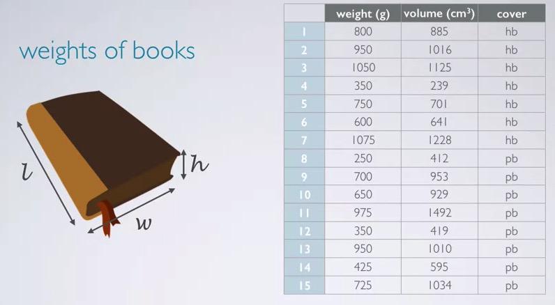
Screenshot taken from Coursera 00:33

In this example, we want to use volume and cover(hardcover/paper) as our explanatory variable, the predictor, to predict weight, the response variable.

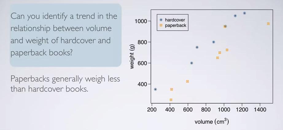
Screenshot taken from Coursera 01:19

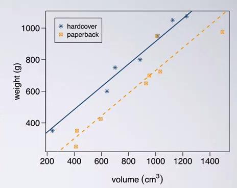
Plotting in the scatter plot, we can see the difference in weight for hardcover vs paperback. Hardcover are generally weigh more than the paperback.

This data currently live in DAAG R library. So let's load that and perform summary of multiple linear regression.

#load data
library(DAAG)
data(allbacks)

#fit model using lm (#response# ~ #explanatories#, #data#)
book_mlr = lm(weight ~ volume + cover, data = allbacks)
summary(book_mlr)

Call:
lm(formula = weight ~ volume + cover, data = allbacks)

Residuals:
    Min      1Q  Median      3Q     Max 
-110.10  -32.32  -16.10   28.93  210.95 

Coefficients:
              Estimate Std. Error t value Pr(>|t|)    
(Intercept)  197.96284   59.19274   3.344 0.005841 ** 
volume         0.71795    0.06153  11.669  6.6e-08 ***
coverpb     -184.04727   40.49420  -4.545 0.000672 ***
---
Signif. codes:  0 ‘***’ 0.001 ‘**’ 0.01 ‘*’ 0.05 ‘.’ 0.1 ‘ ’ 1

Residual standard error: 78.2 on 12 degrees of freedom
Multiple R-squared:  0.9275,	Adjusted R-squared:  0.9154 
F-statistic: 76.73 on 2 and 12 DF,  p-value: 1.455e-07

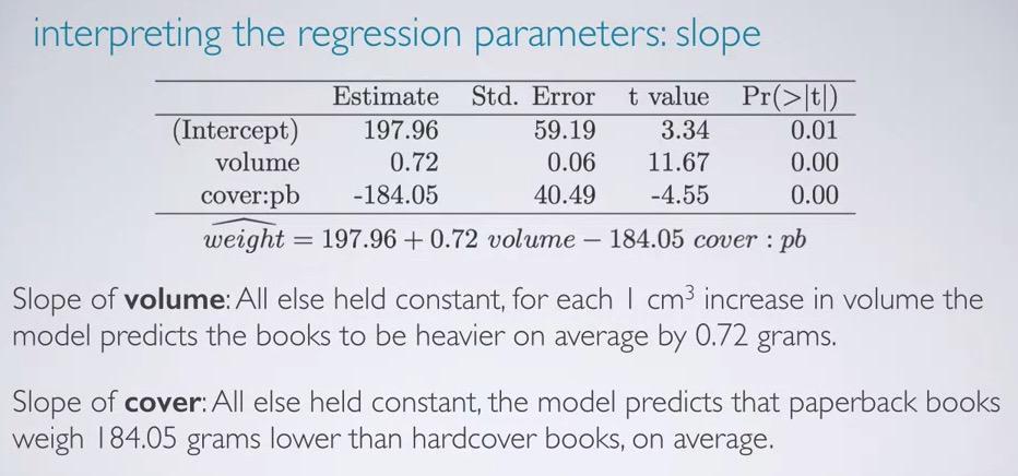
In this summary we can see MLR output. Remember the reference level is a label that's not in the context. In this case, cover lacks hardcover, which means hardcover is the reference level for cover. So we can see that we have 92.75%, which is percentage of variability in weights can be explained by the volume and cover type books. This is a good model, and it seems weights and cover type capture most of features, where the residuals can be caused by unexplained explanatory variables.

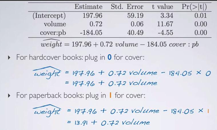
Screenshot taken from Coursera 05:25

Using earlier informations as a basis, we can simplify our MLR into single line for each category. Recall that the hardcover is the reference level for the cover, we can eliminate the coverslope and get our predictor for hardcover books. Same goes for paperback, we can include the slope cover and get paperback predictor. The results is very intuitive, as you can see from the intercept, paperback weigh less than the hardcover.

Screenshot taken from Coursera 06:07

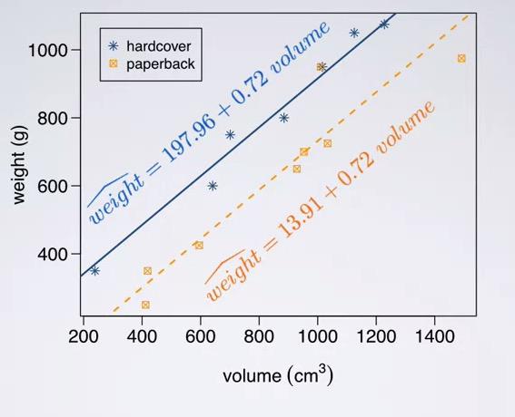
Notice that we have multiple linear regression in our plot, instead of imposing one line that's trying to conclude both level in cover. This way we get a more accurate predictor.

Screenshot taken from Coursera 08:06

So how do interpret the slope? Here we have new statement, All else held constant. What it mean is given that in case all other variables are constant, we want to focus just one explanatory variable, in this case the volume. Recall that the interpretation for numerical explanatory is that given 1 unit increase in explanatory, response will be higher/decrease based on the units. Since the volume is in cm3 for units, and weight is in grams, we can intercept the slope as All else held constant, for each 1 cm^3 increase in volume, the model predicts the books to be heavier on average by 0.72 grams.

And what about the cover? Remember that the hardcover is the reference level, like explanatory in categorical, we say All else held constant, the model predicts that paperback books weigh 185.05 grams less than hardcover books, on average.

Screenshot taken from Coursera 08:54

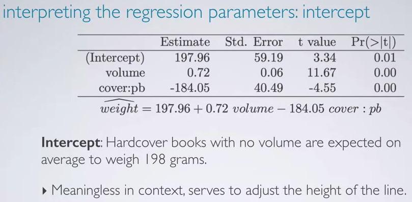
So this is how we interpret the intercept. If all set to zero, (in this case the categorical refer back to reference level), hardcover books with no volumes are expected on average to weigh 198 grams. This is meaningless, as it's not possible of books with no volumes. But it's still serve to adjust the height of the line.

Screenshot taken from Coursera 09:42

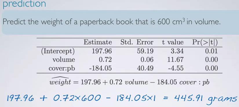
And for prediction we can just plug in all explanatory variable,calculate using the formula and we get the weight.

Interaction variables

Screenshot taken from Coursera 10:53

Note that the books example are oversimplifying example. We assume the slope to be the same for hardcover and paperback. And this is not always the case. interaction variable have to be use in the model, but it's not going to be discussed here.

Adjusted R Squared

Screenshot taken from Coursera 01:42

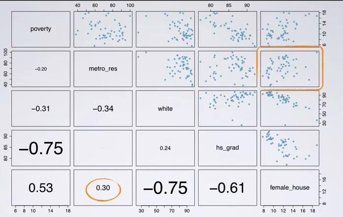
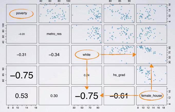
Recall in my blog post earlier we're talking about predicting poverty with HS graduate, here we have a scatter matrix, that can plot for each relationship, and correlation coeffecient.Loading the dataset(the dataset is taken from Data Analysis and Statistical Inference, at Coursera)

states = read.csv('http://bit.ly/dasi_states')

head(states)

       state metro_res white hs_grad poverty female_house
1    Alabama      55.4  71.3    79.9    14.6         14.2
2     Alaska      65.6  70.8    90.6     8.3         10.8
3    Arizona      88.2  87.7    83.8    13.3         11.1
4   Arkansas      52.5  81.0    80.9    18.0         12.1
5 California      94.4  77.5    81.1    12.8         12.6
6   Colorado      84.5  90.2    88.7     9.4          9.6

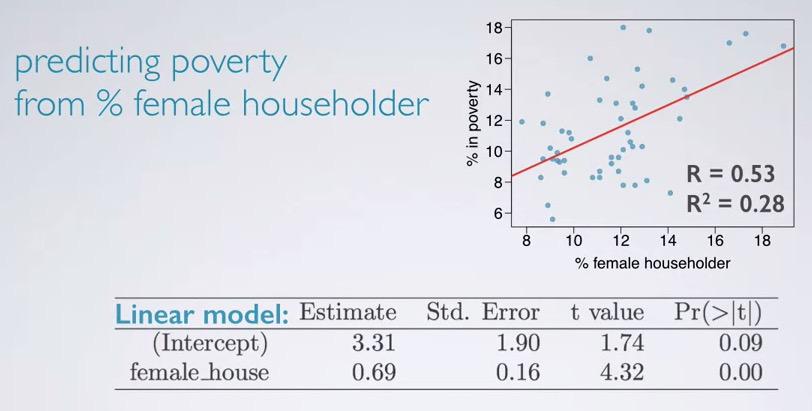
Next, we're going to fit the model, using female_house as the only explanatory variable.

pov_slr = lm(poverty ~ female_house, data=states)
summary(pov_slr)

Call:
lm(formula = poverty ~ female_house, data = states)

Residuals:
    Min      1Q  Median      3Q     Max 
-5.7537 -1.8252 -0.0375  1.5565  6.3285 

Coefficients:
             Estimate Std. Error t value Pr(>|t|)    
(Intercept)    3.3094     1.8970   1.745   0.0873 .  
female_house   0.6911     0.1599   4.322 7.53e-05 ***
---
Signif. codes:  0 ‘***’ 0.001 ‘**’ 0.01 ‘*’ 0.05 ‘.’ 0.1 ‘ ’ 1

Residual standard error: 2.664 on 49 degrees of freedom
Multiple R-squared:  0.276,	Adjusted R-squared:  0.2613 
F-statistic: 18.68 on 1 and 49 DF,  p-value: 7.534e-05

And here we see the R squared.

Screenshot taken from Coursera 03:30

Take a look and see how the data plotted and also the linear model is there. Looking at the p-value approximate to zero, meaning the female house is a significant predictor to the poverty.

Screenshot taken from Coursera 03:31

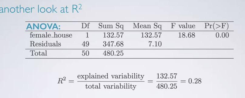
Once, we can also do it from ANOVA table, and we have 0.28.Now what if we're adding one feature, in this case white?

pov_mlr = lm(poverty ~ female_house + white, data=states)
summary(pov_mlr)

Call:
lm(formula = poverty ~ female_house + white, data = states)

Residuals:
    Min      1Q  Median      3Q     Max 
-5.5245 -1.8526 -0.0381  1.3770  6.2689 

Coefficients:
             Estimate Std. Error t value Pr(>|t|)    
(Intercept)  -2.57894    5.78491  -0.446 0.657743    
female_house  0.88689    0.24191   3.666 0.000615 ***
white         0.04418    0.04101   1.077 0.286755    
---
Signif. codes:  0 ‘***’ 0.001 ‘**’ 0.01 ‘*’ 0.05 ‘.’ 0.1 ‘ ’ 1

Residual standard error: 2.659 on 48 degrees of freedom
Multiple R-squared:  0.2931,	Adjusted R-squared:  0.2637 
F-statistic: 9.953 on 2 and 48 DF,  p-value: 0.0002422

anova(pov_mlr)

Analysis of Variance Table

Response: poverty
             Df Sum Sq Mean Sq F value    Pr(>F)    
female_house  1 132.57 132.568 18.7447 7.562e-05 ***
white         1   8.21   8.207  1.1605    0.2868    
Residuals    48 339.47   7.072                      
---
Signif. codes:  0 ‘***’ 0.001 ‘**’ 0.01 ‘*’ 0.05 ‘.’ 0.1 ‘ ’ 1

We can calculate our R Squared from ANOVA table,

ssq_fh = 132.57
ssq_white = 8.21
total_ssq = 480.25

(ssq_fh+ssq_white)/total_ssq

[1] 0.293139

And the result is the same with p-value from linear regression. Since this is the proportion of variability poverty that can explained by both explanatory variables, female_house and white, for female_house only contributed female house, the proportion is only incorporate the female_house, which in this case:

ssq_fh/total_ssq

[1] 0.2760437

Screenshot taken from Coursera 07:36

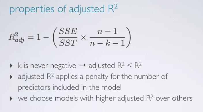
As we increase our features, our R squared is increase as well (attributed by dof). So, we also want to know whether additional feature is significant predictor or not. And for that, we use adjusted R squared. The value will add a formula which incorporate the number of predictor. If the new R squared can't offset penalty of number predictors, the additional feature will be excluded.

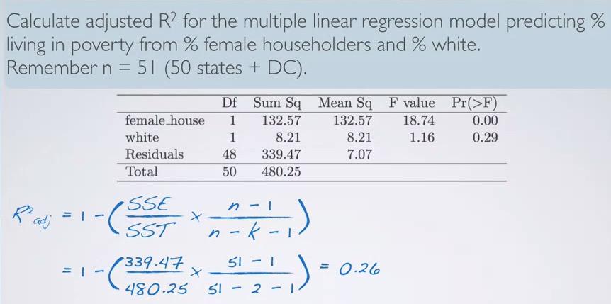
Screenshot taken from Coursera 08:40

The sample size is 51 (50 states + DC). And the explanatory total is 2, fh and white, so we have n and k. Plugging those into the formula, incorporating SS residuals(unexplained), SS total, n and k, we get 0.26. So this will means that the additional predictor is getting penalty, and may not contributed significantly to the model.

Screenshot taken from Coursera 09:18

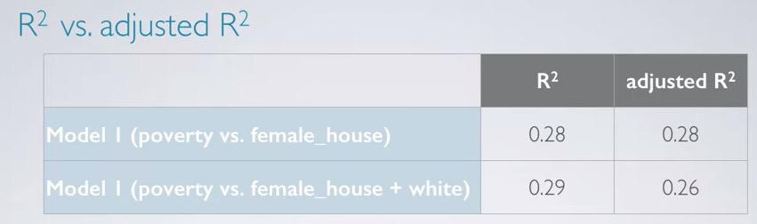
In the previous model where we only have one explanatory variable, R squared not getting penalty, as shown by same value for both R squared and adjusted R squared. However, after the model add new predictor, white, R squared increase(remember it will always increase as the predictor added), but adjusted R squared is not increase, even decrease. This would means 'white' isn't contributed to the model significantly.

Screenshot taken from Coursera 10:00

So since k is never zero or lower, It impacts the adjusted R squared being smaller. But still adjusted R squared is the more preferable than the others.Remember this is still doesn't change the fact that R squared is proportion variability of response that explained by the model, and this what's not adjusted R squared definition.

Collinearity and Parsimony

Collinear

Two predictors are said to be collinear when they correlated with each other. Since the predictor is conditioned to be independent with each other, it's violated and may give unreliable model. Inclusion of collinear predictors are called multicollinearity.

Screenshot taken from Coursera 02:15

Earlier we have incorporate 'white' as our second predictor, and turns out R squared is not changed, even getting penalty by adjusted R squared. Looking at parwise plot once gain, we can infer from the correlation coeffecient and scatter plot, that both variables are strong negative correlation. This will bring multicolinearity which will disrupt our model. So we should exclude 'white' on this. And that conclusion will bring us to parsimony.

Parsimony

By avoiding features that correlation with each other, we actually do parsimony. The reason to exclude the feature is because it's not bring useful information to the model. Parsimonious model are said to be the best simplest model. It arises from Occam's razor, which states among competing hypothesis, the one with fewest assumption should be selected. In other words, when the models are equally good, we avoid the model with higher number of feature. It is impossible to control feature in observational study, but it's possible to control it in the experiment.

In the machine learning field, it often useful to exclude those features. First as we avoid them, we also avoid curse of dimensionality, which states the learning will take longer exponentially, with huge number of features. So features(predictor) selection is what we're trying to use. It also avoid variance in our model that tend to overfitting, make it harder to generalize to the future problem.

In summary:

we can define MLR as ,

$$\hat{y} = \beta0 + \beta1x1 + .. \beta{k}xk$$

where k = number of predictors and x as the slope.

As for the interpretation of MLR, for the intercept we're assuming that all explanatory being zero, what are the expected value of the response variable on average. For the slope, assuming all else being equal, for each unit increase in particular (1 unit) explanatory, we expect the response to be increase/decrease on average by {explanatory slope}.

In MLR, we want to avoid two explanatory variables that dependent. Because it will mitigate the accuracy of our problem. One way to avoid this is to select one of the variables, or merge it into one (pca).

R squared will alwayws getting higher as you increase variables. To make it more robust, we use adjusted R squared, which give penalty to those features that doesn't provide useful information to the model.If it does, the model should have higher adjusted R squared, instead of getting constant or even decreasing the R squared. using the formula,

$$R_{adj}^2 = 1 - \frac{SSE / (n-k-1)}{SST/(n-1)}$$

where n is the number of observations, and k as the number of predictors

Lastly, we want the model to parsinomous model. That is the model with the best accuracy, but also with the simplest model. Full model is where we use all the explanatory to predict the response, and we can mitigate the variables using model selection, which we will be discuss with my next blog.

REFERENCES:

Dr. Mine Çetinkaya-Rundel, Cousera