Confidence Interval
Confidence Interval (CI)
Confidence interval is the range of plausible values in which we want to capture the population parameter. For example if estimate the point estimate, if we guess the exact value chances are we will miss. But if we take range of plausible values (net fishing instead of doing it with spear), there's a good chance that we capture population parameter.Note that sample statistics acts as a point estimate to our population parameter. So if we want to get a population mean, we get a point estimate mean. In this case, the sample statistics and point estimate is synonymous.
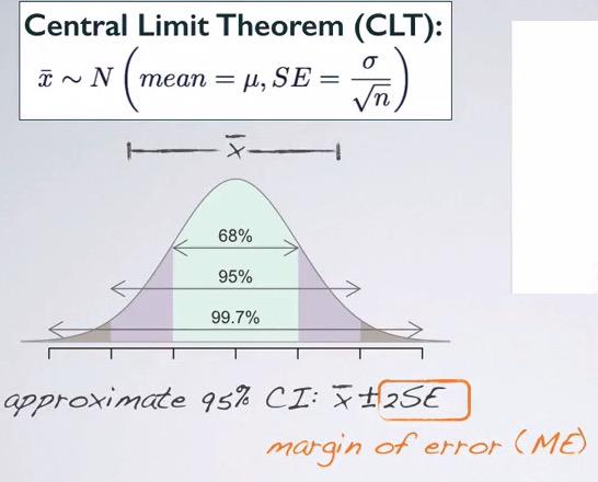
Snapshot taken from Coursera 02:53
So typically CI is within two standard error, within 95% of sampling distribution. The question really is, when we take sample and calculate the point estimate, the mean, what is the probability that the mean of the sample is within two standard deviation of sampling distribution. Remember $\bar{x}$ is our mean sample. So there are two mutually exclusive events here. Either the sample mean within 95% CI, or it doesn't.Remember that within 95% means within 2 standard deviation.Half of this range is often called margin of error (ME).
CLT have its own requirement, if point estimates is about mean:
- Assert that population distribution is normal. If we can't check that, we can infer from the shape of sample distribution taken.
- The sample size >= 30 or population distribution is normal, larger if the distribution is more skewed.
- The samples taken is independent.
- the distribution of sample mean will be nearly normal, and we can calculate with CLT advantage.
- The larger the sample size, the less concern it will be about the shape of population distribution.
If the sample is taking by random sampling/assignment, and the sample size is less than 10% of population, then CI can take advantage of CLT. Sampling distributions that doesn't support CLT skew,size, and independence will not be normal.
Let's take a look at one of the example.
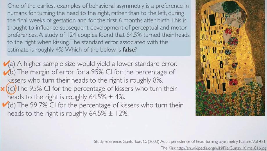
Snapshot taken from Coursera 06:17
In this study, we can find the following:
$\bar{x}$ = 64.5%
$\sigma$ = 4%
So the first example is always true. Conceptually, the higher the sample size, the less variability of error, led to lower standard error. Mathematically, taking formula for calculating of standard error, inversely, sample size increase, will decrease the standard error.
The second example is also correct 95% means two standard deviation, give us Margin of Error:
two standard deviation * 2 = 8%
Third case, as we said earlier, two standard deviation, but this example only gives us 1 standard deviation, hence it's not correct. The final options is true. Although it's different level of confidence, it's also valid. within 99.7% would means 3 standard deviaion hence:
3*sd = 12%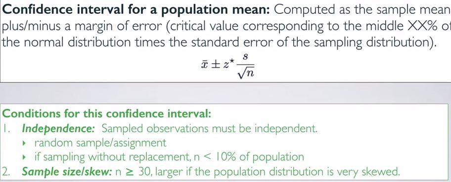
Snapshot taken from Coursera 08:17
So because the CI is based on the CLT, CI has same requirements, though stricter. For the skewness, CLT let's you at least more than 30 size of the sample. But CI on the other hand require larger size if the population is very skew. Here we see that any interval is correct, as long we specify the standard error accordingly.Again we use s to denote standard deviation of sample distributions. Since we're almost always doesn't get true population mean, we use mean of sample.
Note that because we also use z-score in conjunction with the SE, that doesn't mean standard deviation is similar to standard error. $\sigma\$ is used to describe the variability of your data. While SE is used to decribed the error variety of your samples point estimates, taken with same size and from the same population.
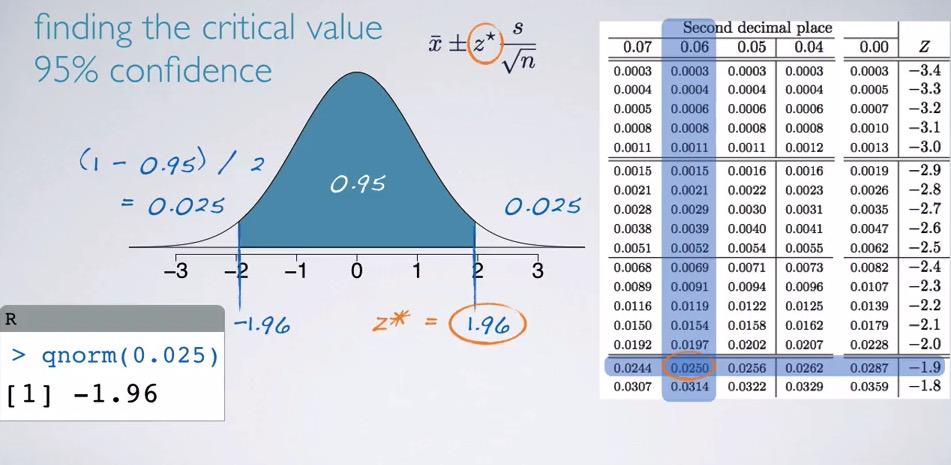
Snapshot taken from Coursera 11:02
So we know that 95% is only approximate to 2 standard deviation. We're doing that because we want to rounding up. Taking the exact standard deviation will need calculation above. We can simply take half of the proportion, cutting the distribution and finding what are the standard deviation. Since we're doing qnorm without specifying the lower.tail, it will give the lower tail hence left standard deviation. Critical value is always positive, and for right standard deviation, we only need to make it positive value.
Accuracy vs Precision
Snapshot taken from Coursera 02:06
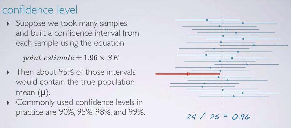
Taking the plot above, we know that 95% is famous for CI with 1.96SE. But it could also work well with 90%,98%,99%. Suppose we take same sample size and plot it 25 times. It turns out, one sample in its interval is not capturing true population. In this case what we get is 24/25 = 0.96. Note that because it is sampling, and therefore have sampling variability, there's a chance that our sampling doesn't catch point estimate, population mean for example.
Snapshot taken from Coursera 03:17
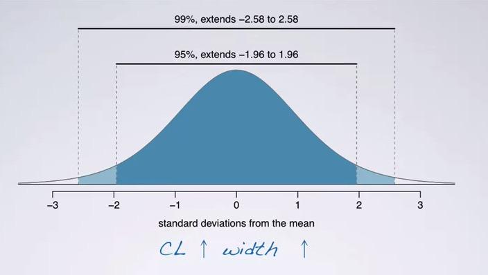
Increase the confidence level, will increase the range of the interval as well. as The level gets higher, the interval is also get higher. We see that plot above, 95% will take all data within 1.96 deviations, 99% will take all data within 2.58 standard deviation. Sadly it's no free lunch, it comes with a cost.
So we're going to compare the accuracy vs precision.The accuracy is about whether we're exactly predicting the value, the precision is about the width of the interval. Suppose we're predicting a value based on Confidence Interval. Is the value that we get is precise? Basically no. So as the higher confidence level, the lower the precision.Why? Because as we increase the confidence level, our standard error is also increase, that is the width of our interval. So how we get best of both worlds? We increase the sample size. As we get higher the sample size, the variability of error(SE) will decrease.This would means get lower precision.
Snapshot taken from Coursera 07:17
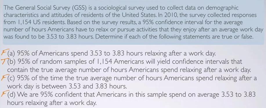
- a is False. This is not about observing the individuals, rather, the population parameter, the average.
- b is True. This is the exact definition of the confidence interval
- c is False. this is not the probability in which one events occurs between certain range vs they dont. 95% is the interval, not probability. Saying 95% probability that occurs in a range 3.53-3.83 is not correct.
- d is False. Confidence Interval is not talking about the sample, it's talking about the population parameter. This would be correct if it's said 100% confidence, because that's what we are getting sample mean as a basis of CLT. But getting sample mean only is not truly interesting.
So in summary:
- We can say something like 'We are 95% confident that true average population have been between this and this'
- We can say that 95% of random samples with same size and from same population will yield an interval that capture the true population parameter.
- We can say confidence interval will capture true population parameter.
- We can say 95% is the percentage of random samples that capture true population parameter.
However:
- we can't say '95% of the time, true average lies between ..', this is not a probability.
- we can't say '95% of the samples will have average between ...', CI is about the true population parameter, not sample.
Master statement CI from various problem will help you through various problem.Always mention what your population is and the parameter.
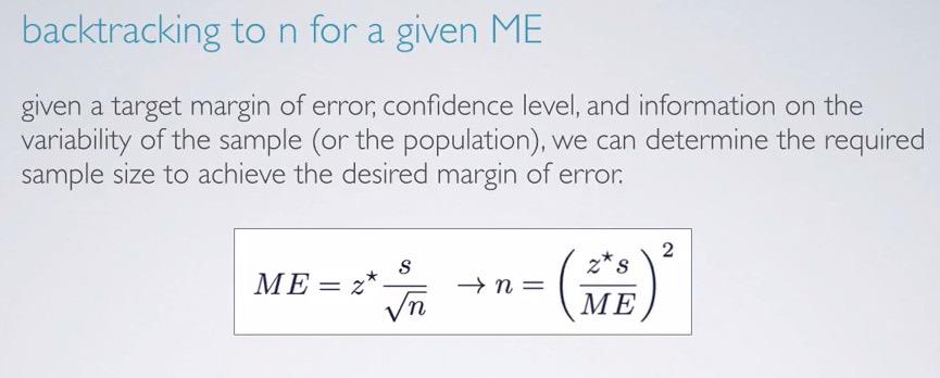
Required sample size for ME
Snapshot taken from Coursera 00:44
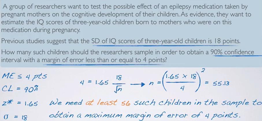
Consider following example where we can plug everything in.
Snapshot taken from Coursera 03:21
We know that the margin of error should at maximum 4, can't go any higher than that. Getting critical value for 90% confidence level can be done as:
(1 - 0.9)/2 = 0.05%R qnorm(0.05)
So we get approximately 1.65 (if using z-table). Now that we have everything in our hand, calculating the sample size should be easy. The result that we get is 55.13. But since we're calculating people here, desimal should not be in place. As the result stated the minimum value is 55.13, rounding down would be mistake in statistics, eventhough it should be mathematically. As this is the requirement, we have to always round up to nearest value, therefore 56. Notice that the relationship between sample size and ME is inverse exponential. Half the margin of error, we have to increase to quarduple the sample size. This confirm the CLT earlier, where if you want 1/3 margin of error, you have to multiply n by 9.
The Z-score that we get is negative, but it's only a sign that the calculation observe the lower tail. So as distance is absolute number, you convert it to positive. Say, what you concern is only one-tail, that is less than, not greater than. Why we still divide it by 2? Because no matter one/two tail, CI will always symmetric, that is you always concern about two tails, eventhough you only consider one tail.
CI(Mean) examples

Snapshot taken from Coursera 01:21
Remember that the confidence level is about what the population mean reallys is, and the interval which capture the data. So we can say, 'We are 95% confident that Americans on average have 3.40 to 4.24 have bad mental health days per month.'
Here another question. In this context, what does a 95% confidence level mean?
If we're able to capture the mean of confidence interval through various problem, then you're able to master the material.Remember that confidence interval was achieved through gather samples with same size and from same population, plot it into sampling distribution. we can say that 95% of random samples of 1151 Americans will have CIs that yields interval that capture the true population average of bad mentah health days.
If researchers found 99% interval is more appropriate, is the interval wider or narrower?
Wider of course.Depending of your error, if you don't want to increase the standard error, you should increase your larger size exponentially.

Snapshot taken from Coursera 04:26
All the condition are met. We know the sample size, the mean, and standard deviation. But first, we must checked at the conditions.
- The sample never stated by random sampling. But 50 is less than 10% of college students. By checking that, we have good assumption that the sample is independent.
- n > 30 & not so skewed sample.Knowing that 50 is more than 30, we can make assumption the sampling distributions will be nearly normal.
After confirming those, we can make a calculation.
Let's us state that:
n = 50
mu  =  3.2
s = 1.74
z = 1.96
$$SE = \frac{s}{n} = \frac{1.74}{\sqrt{50}} \approx 0.246$$
$$\bar{x} \pm z * SE = 3.2 \pm 1.96 * 0.246 $$
$$3.2 \pm 0.48 = (2.72,3.68)$$
So we are 95% confident that true average of mutually exclusive college students have been in 2.72 - 3.68 exclusive relationships
Margin of error is half the confidence interval, so the distance between the middle of interval to either direction.
REFERENCES: