Introduction to Statistical Distributions
Normal Distribution
Normal Distribution will is the distribution which calculates popularity of the population. This will get discussed on including standard deviation to determine Z score of particular value.
Screenshot taken from Coursera video, 01:57
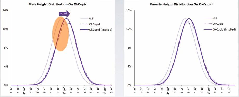
This distribution shows the distribution for both male and female, with height repored on the U.S survey and OkCupid. The height distribution of OkCupid is slightly to the right, which can be told as people often over-exaggerated their heights/tends to round up the height to the top.
Many data is not exactly shape like a bell-curve, as its represent the real data, it's natural that it's nearly but not exactly normal. But when you see that the distribution tends to like bell-curve, we can assume the distribution is normal distribution, an unimodal. A normal distribution will make all data distributed around center, the mean.
Screenshot taken from Coursera video, 05:29
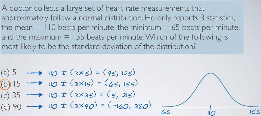
The fact that the questions include the data to have normal distribution, is our critical information. A normal distribution should have all data that are in 3 standard deviation, 99.7%. With that in mind, because we are given 3 statistics value, we can predict the standard deviation that closely match the minimum and maximum. Turns out the answer (b) has matched the criteria perfectly.
Screenshot taken from Coursera video, 06:29
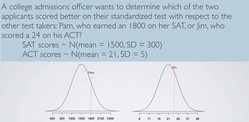
This is one of the example of standarized test. Instead of comparing raw score, which would give Pam absolute winning, we can calculate Z-score, which tells us the both scores in their respective standard deviation away from the mean.
Screenshot taken from Coursera video, 07:20
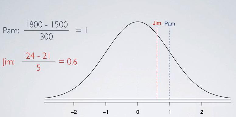
Plotting all of the value in standarized distributin, we see clearly that Pam has higher value from Jim.
Screenshot taken from Coursera video, 09:03
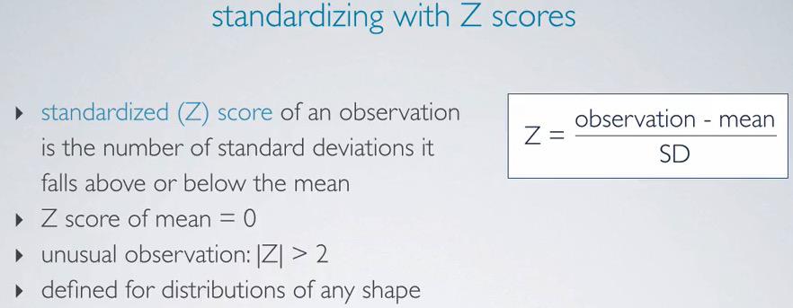
The Z score comes from letter z in 'standardizing', s has taken for 'standard deviation'. Z score of the mean is simply 0, because it only subtracting for the mean value iself.
When the distribution is converted to the standardized Z score, the mean will be 0, and the median will roughly 0 as well, because it's normal distribution.When you're standardizing, it's not take the original distribution, rather standardized distribution, which is exact normal distribution centered at 0. Therefore positive skewed will give you negative median, negative skewed will give you positive median.
Z-scores can also be used to calculate percentiles, which is the percentage of population below the mean. Other's distribution can take percentile as well, as long it's unimodal. But those will require us to using extra calculus.Note that this means regardless the shape or skew of the distribution, z can always be defined, provided mean and standard deviation. But this doesn't mean we can compute percentiles, percentiles distribution need normalty.
We can easily using R to specify the what value that we want to observe, the mean, and the value of standard deviation using R
%load_ext rmagic
%R pnorm(-1, mean=0, sd=1)
Screenshot taken from Coursera video, 14:37
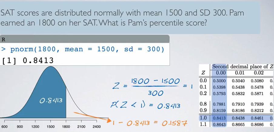
This question can be arrived at solving it in R or by using percentage. Note that we can also counting the percentiles manually but it's not recommended. We already know 68%-95%-99.7%, and we know that below standard deviation of 1 is roughly 84%.Using R:
%R pnorm(1800, mean=1500, sd=300)
This will answer that Pam's score is better than 84% of her class. We always calculate the percentiles below the value. To calculate who's better than her, we just calculate the complementary, which resulting in 0.1587
%R pnorm(24,mean=21,sd=5)dd
0.9*2400
Screenshot taken from Coursera video, 17:17
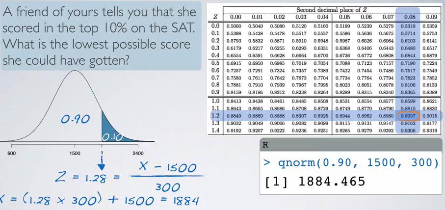
Using this we can determine the X value, in R, we're using different method. Given quantile/percentile that is cut, we're trying to predict the value that resides there. Note that because she's in top 10% we cut 10% from the top.
%R qnorm(0.90,1500,300)
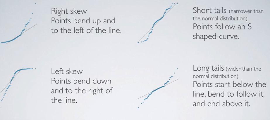
Evaluating Normal Distribution
Screenshot taken from Coursera video, 00:15
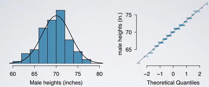
This is the usual plotting histogram and scatter plot to validate if the population indeed has normal distribution.
Screenshot taken from Coursera video, 01:23
Screenshot taken from Coursera video, 02:44
We can also checking the spread of the distribution by plotting standard deviation. If the spread of the distribution in 1 standard deviation is higher than 68% (normal distribution in 1 standard deviation), it's expected that the distribution has more variable, more spread.
Normal Distribution Example
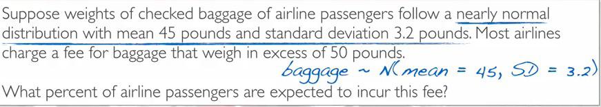
Screenshot taken from Coursera video, 00:41
revans = %R pnorm(50,mean=45,sd=3.2)
1 - revans[0]
5.9% passengers are expected of excess the bagage.
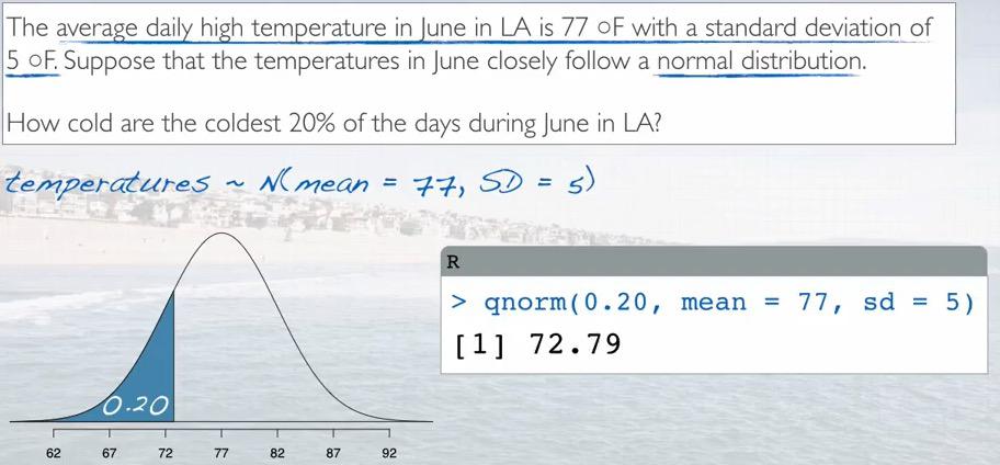
Screenshot taken from Coursera video, 04:06
%R qnorm(0.2, 77, 5)
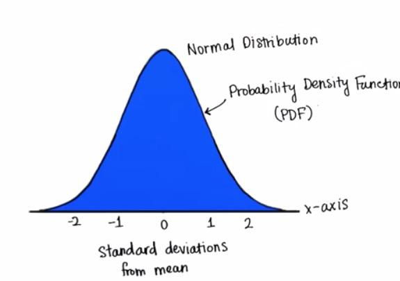
Screenshot taken from Udacity video, 00:36
Remember that sum of normal distribution, because it all based on relative frequency add up to 1? That's called Probability Density Function (PDF).
In this way, because all of the relative frequency add up to 1, we can treat it the same as the probability
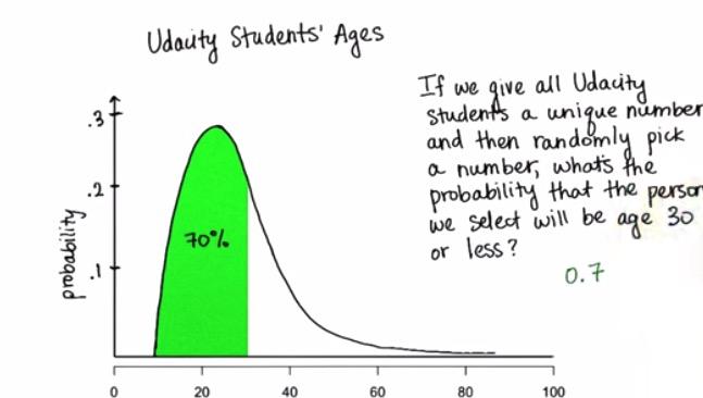
Screenshot taken from Udacity video, 00:12
In normal distribution, the two-tail is never touch the x-axis(horizontal asymptote). That's because we can never be sure at 100%. If the distribution touch at x-axis, then it equals 1, however the PDF just close to 1, even it extend to 5 standard deviations away.
The green area is the probability of randomly selecting less than the threshold, which in turn proportion in sample/population with score less than the threshold. So you see, the two-tail actually goes to infinity.
0.95-0.135
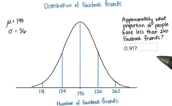
Screenshot taken from Udacity video, 00:12
%R pnorm(240,mean=190,sd=36)
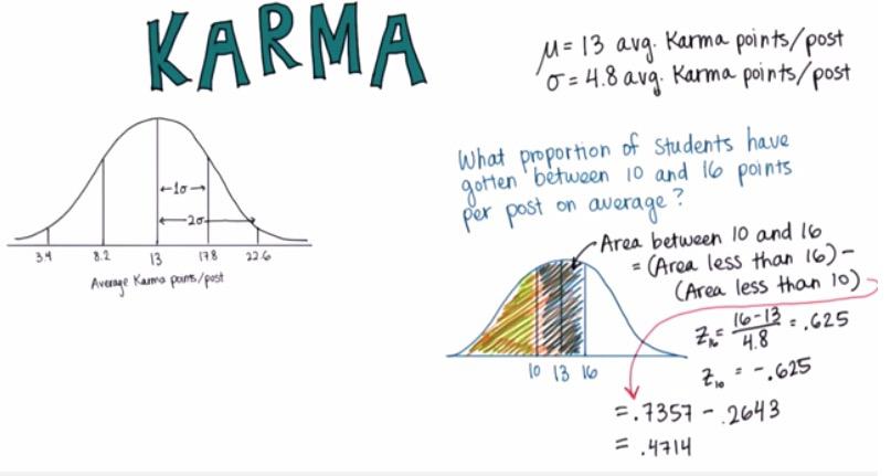
Screenshot taken from Udacity video, 02:09
a = %R pnorm(16,mean=13,sd=4.8)
a = 1-a[0]
b = %R pnorm(10,mean=13,sd=4.8)
1.0 - a - b[0]
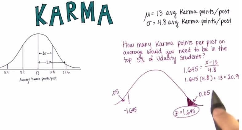
Screenshot taken from Udacity video, 02:09
%R qnorm(0.95,13,4.8)
Sampling Distributions
We know how we can compare between two normal distribution. But how about sample distributions? How can we compare of one sample with the other sample within that population? We can:
- find the mean of the sample
- find other means of other samples
- And we can compare all the means from samples.
If we're using thethral die, and roll 2 times, it would mean we're sampling size 2 out of our population, resulting in 2^4 = 16 total possibilities.We can take means of all sampling possibilities.After that, if we take average of all means possibilities, we get Means that equals to the means of the population.This all sample means that we get from the means of sample size 2 possibilities.
Mean of each sample: 1, 1.5, 2, 2.5, 1.5, 2, 2.5, 3, 2, 2.5, 3, 3.5, 2.5, 3, 3.5, 4
When we average this, we get 2.5, equals to means of the population. So the mean of each sample is the mean of the population. This will taking an advantage of sampling, because it's often the case where population is too large and we're short on computing because the data is too big.
If we copy this to web http://www.wolframalpha.com/:
We get a histogram plot for this data. The data, a sample means, is actually a distribution itself which often called Sampling Distributions.
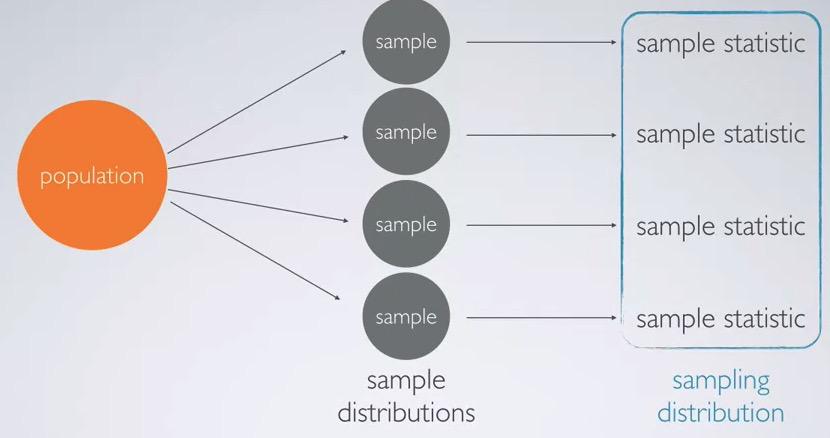
Snapshot taken from Coursera 02:57
Let's take another look. Earlier we're take inifinite number of sample possibilities. But that's just extreme condition. The everytime we take sample from the population we have sample distributions. And for example we're taking sample statistic, in this case, the mean. Plotting mean into the distribution would be called sampling distribution. So there's different between sample distributions and sampling distribution.
Snapshot taken from Coursera 04:07
But we're missing some important point. What do we need to compare mean in a single sample with other sample's mean in the distribution? We don't know whether the mean of the sample that we took will be located in which location of Sampling Distributions. In this case, we need Standard Deviation.
Note that because we're using sample means as our data, doesn't mean we need to use Bessel's Correction(n-1). We already have all the possible outcomes, and that's the entire data of our population(means sample).What we're calculating is not actually standard deviation, the standard deviation of all possible sample means is called Standard Error.
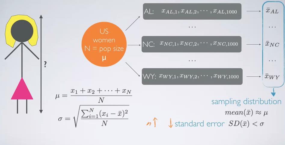
In the case above we're taking 1000 sample for each of the state. This problem arise to know the population height of all women. Suppose we know the sample size, the mean, and all height of women population in the US. Then we do that sampling distribution, collecting mean for each of sample state.The mean of sample distribution should approximately equal to the mean of population.The variability should be less than variability of the population, since the population outliers are outliers combining for all states.
Screenshot taken from Udacity video, 00:23
There's actually a relationship between standard deviation of population and standard error,
$$ SE = \frac{\sigma}{\sqrt{n}} $$
- $\sigma$ = population standard deviation
- SE = Standard Deviation of distribution sample means
- n = sample size
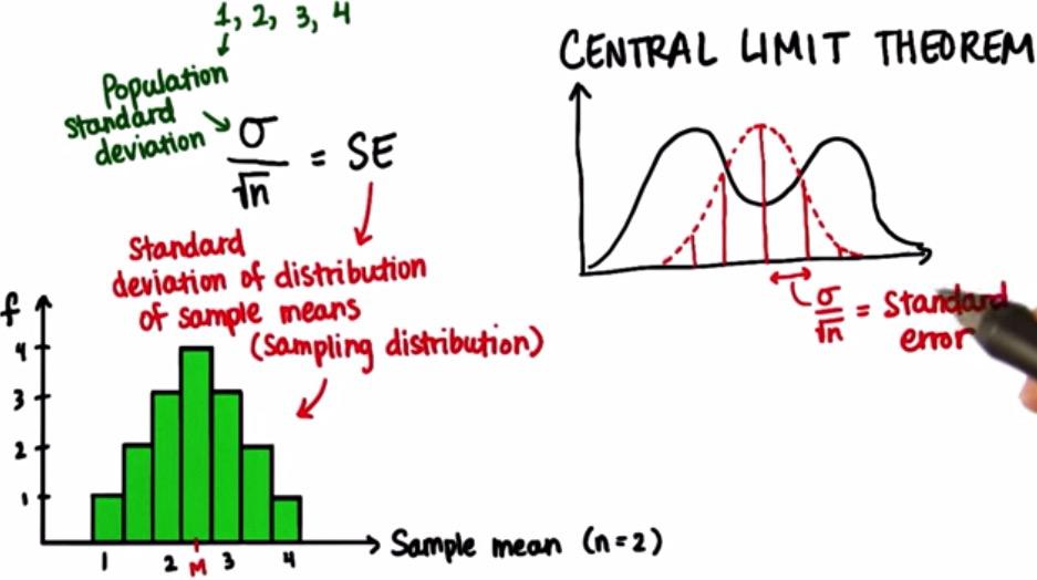
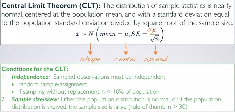
This solve the original problem, which require us to find where the sample lie on distribution of sample means.This called Central Limit Theorem,that if you keep fetching fix sample size(n) all possible sample outcome, you're getting normal distribution that has standard deviation that equals Standard Error. Turns out the Standard Error is not easy to get, because that's mean we have to have all population data. And for that there's mathematical formula which stated above.
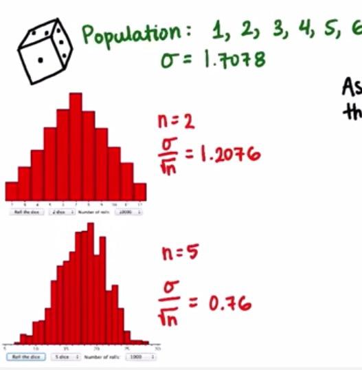
Screenshot taken from Udacity video, 00:23
Note that as we grow the sample size, the sampling distribution will get skinnier. This can be proved by mathematical formula earlier, sample size bigger will make bigger value in the denominator, that makes smaller standard error, hence skinnier sampling distribution.
Intuitively, as the sample size bigger, the variety about where the mean of entire population get smaller, we get better prediction. To achieve half the mean error of the sampling distribution, we have to quarduple the sample size, 4xn, which we can replace it to the formula earlier to prove it.To get the error 1/3 from before we need:
$$ \frac{1}{3} . \frac{\sigma}{\sqrt{n}} = \frac{\sigma}{\sqrt{9n}}$$
The important thing to take away, is that when you're sampling to any distribution and distributed all the possible means, you will get aprroximately a normal distribution. As you're sample size bigger, the error will get smaller and converge to actual mean. This can get very intuitive. In the extreme condition, when your sample size match the size of the population, you will get the exact mean of the population.Keep in mind, that if you're averaging all possible means no matter what sample size, you're should get approximately the mean of the population.
Snapshot taken from Coursera 12:55
This is more official definition of CLT. Here we saw that the standard deviation is being corrected. Earlier I told you that it's not often the case that standard deviation population can be defined. So instead we can use standard deviation of our sample. In this case, we're using Bessel's correction. The observation must be independent, random sample if observational, or random assignment ifon experiment. To get better intuition for CLT, there's an applet for that http:/bit.ly/clt_mean
The sample size doesn't to be large enough, less than 10 percent if without replacement. We also often don't know the shape of population distribution. If you do sample and turns out the shape is normal, it's more likely that the population which you take sample on is also normal. But to make sure for the distribution we set the minimum of sample size 30.But if you have skew population, high skew for example, then you would need larger sample size to make the shape normal so CLT can works
Why 10% if without replacement? Because too large of sample size would make a larger probability that we grab sample that are dependent one another. For case above, if we're taking 50% sample from women population, chances are there's sibling or related family, and perhaps make similar height because of the genetic, and thus make it dependant. This will disrupt our sample which we want to be perfectly randomised. So not too large, below 10%, but also not too small, above 30.
Snapshot taken from Coursera 17:28
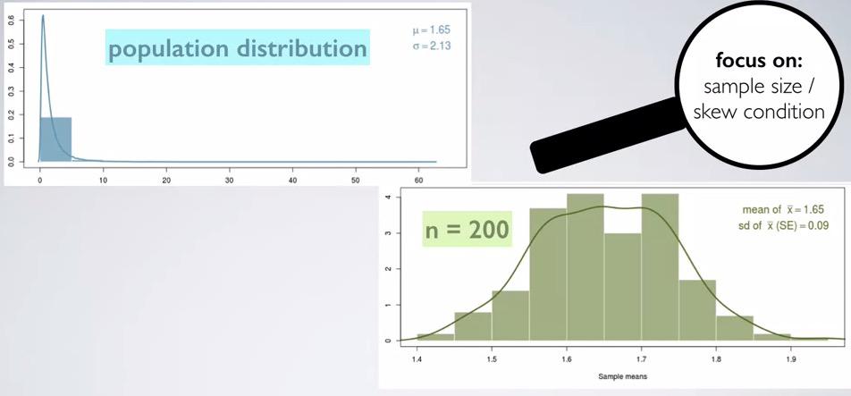
So there's additional reason why the sample size has to be large enough. Consider the population distribution that has right skewed in the case above. When're take sample means and make sampling distribution, it will be like the parent, right skewed. But if take the sample large enough, it will approximate normal distribution. Why we so obsessed about normal shape? Because we need that for Central Limit Theorem to work. CLT will allow many statistical inference to use, including null hypothesis and hypothesis testing to use, which require normal probability distribution. There's also confidence interval that we can use.
Doing z-score that we discussed earlier, we can pretty much calculate the probability in certain distribution.Lower probability would means that certain sampling distribution doesn't affected the whole population.The result of lower probability then, means lower error, and thus not likely to happen by chance.
Let's take an example. There's app Bieber Twitter that may affected Klout Score user. We have the mean, the standard deviation, and number of people, and average score of who uses the Bieber Twitter. From this examples we can extract some information related to Central Limit Theorem.
- Sampling : Bieber Twitter users
- population : Klout Score users
- mean population : 37.72
- sd population 16.04
- avg Klout Score of users that use Bieber Twitter = 40
Suppose that there are 35 Bieber Twitter user.What's the probability that using this app will affected the Klout Score users?
import numpy as np
mu = 37.72
sigma = 16.04
sample_size = 35
SE = sigma/np.sqrt(sample_size)
SE
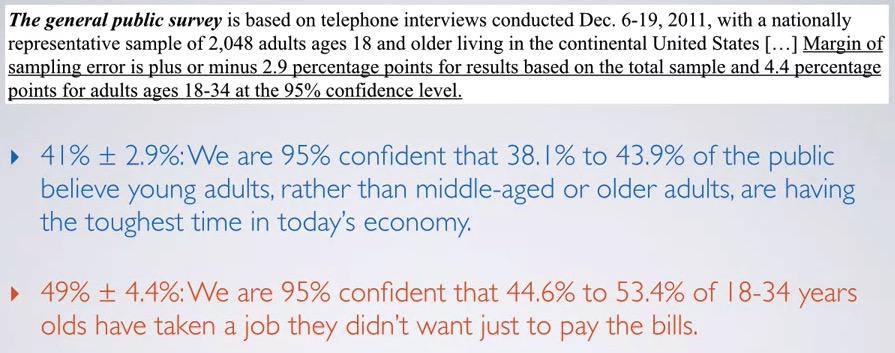
This is our standard error.Average score of Klout population is 37.72. The average score Klout users who use Bieber Twitter is 40. Given this, what's the probability of Bieber Twitter affected Klout Score?
%R mu = 37.72
%R sigma = 2.711
%R pnorm(40, mean=mu,sd=sigma,lower.tail=F)
So doing pnorm tells us that 0.2 probability of using Bieber Tweeter affecting the Kloud Score. There's too much possible reason to mention, but what's important is that our sample is lacking.
Suppose that we increase the sample size to 250,the standard error would be
sample_size =250
SE = sigma/np.sqrt(sample_size)
SE
We can see that we have much smaller standard error from the previous one. Would this increase the probability? What's the Z-score of 40? (mean of sample size 250) Remember that the mean of sampling distribution is exactly the same of mean at entire population.
(40 - mu)/SE
That value means that it's more than 2 standard deviations away, which is very small probability. What's the probability? The probability of randomly selecting a sample with sample size 250 with a mean greater than 110?
%R mu = 37.72
%R sigma =  1.01
%R pnorm(40, mean=mu,sd=sigma,lower.tail=F)
Now please keep in mind, that we plot the mean of this particular sample (of size 250) in the sample means distribution. The probability randomly selecting average at least 40(more than 40, because less will be more common) is very rare, 0.01 if plot it into sampling distributions .This is very unlikely that is random. Things can be due to chance if the probability is still 0.2 like earlier. This explain us that there's maybe some correlation between the app and the Kloud score.Based on this low probability, it's unlikely due to chance.You may not notice this yet, but what we actually do is using CLT for Hypothesis Testing.
So you see, increasing our sample size making our standard error smaller, thus tend to make less error. From our sampling distribution, the mean took from larger sample has lower probability, too low and so rare that is thought not due to chance.The closer the Z-score of a sample to 0 in sampling distribution, the higher the probability that the sample is due to chance.
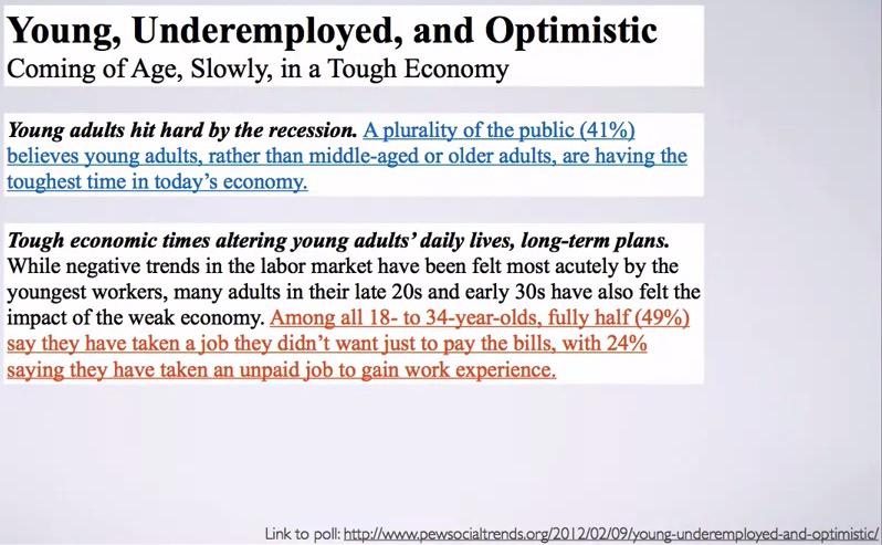
Sampling distribution is also the gate to open Statistical Inference. Consider following case,
Snapshot taken from Coursera 02:57
This data take very expensive resources. Imagine that they have to collect entire data US population. For this, rather than taking population parameters, we're taking sample statistics. As earlier that we've learned so far, we're gonna take all kind of sample in the case, and try to make distribution out of it.
This kind of sample will
In summary, CLT let us know:
- the predicted shape of the distribution (Normal Distribution)
- Expected value of the mean of the distribution (Mean of population)
- Standard Deviation/Standard Error (known from standard deviation and sampling size)
- The bigger the sample size, the smaller standard error, resulted in bigger z-score for that sample mean
- The bigger the z-core,makes skinner distribution, makes less the proportion of sample means greater than that sample mean.
- To minimize the error exactly, we can calculate how much sample size do we need.
- The skewer the shape of the population, the higher sample size that we would need.
- Standard deviation of population is almost always unknown. We can use the sample standard deviation with bessel's correction.
- Point estimates like mean is expected to be equal to mean of the population
- Standard error measures the error variability when we plot sample means into sampling distribution. This to measure the probability of error of our sample. If the probability is low, then it's likely not error and not happend due to chance.This is different than the definition of standard deviation, that measures variability of our data.
CLT example
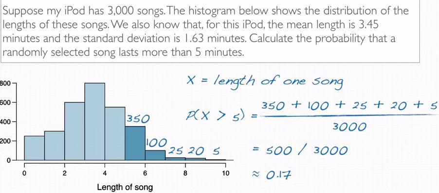
Snapshot taken from Coursera 03:31
This one of the example that later we're going to calculate by CLT. Eyeballing educated guess this problem, we see that by the height of the bar of histogram, we can guess the frequency. Using simple probability calculation, we get approximately 0.17. Using R
%load_ext rmagic
%R pnorm(5,mean=3.45,sd=1.63,lower.tail=F)
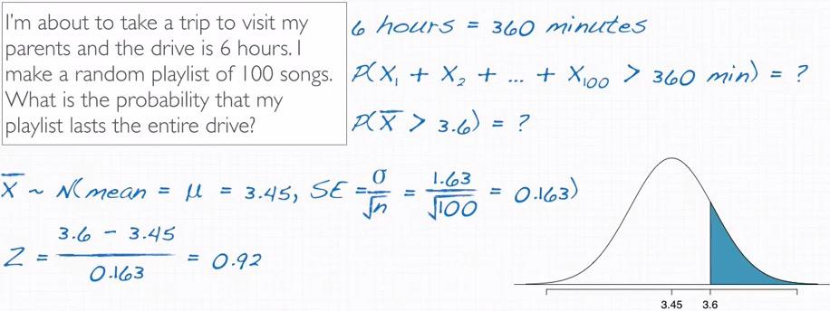
Snapshot taken from Coursera 07:41
Now for this question, we actually taking the average of total 100 songs in ipod that average last at least 3.6 mins.This is not the same as taking probability that each of them last at least 3.6 mins, total the length will be perhaps more than 360 mins.
So we're going to calculate the probability of the skewed distribution. How? by transforming it to normal distribution using CLT. Given mean and standard population earlier, we can make sampling distribution, and calculate the Z-score. Using that, we calculate the probability and have 0.179 using upper tail.Thats the probability that if you randomly select 100 songs, it will last for 60 mins.
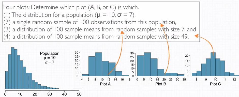
Snapshot taken from Coursera 10:51
Next we're going to match the plot from the probability. Distribution that transform to normal the most is the distribution of sample means that have larger size, in this case right most is 3. The distribution of sample observation, sample distribution but not sampling distribution is in the middle is 2. It also because it resemble right skewed and variability of the original population. The rest is the sampling distribution that have fewer size, left at 1.
Binomial Distribution
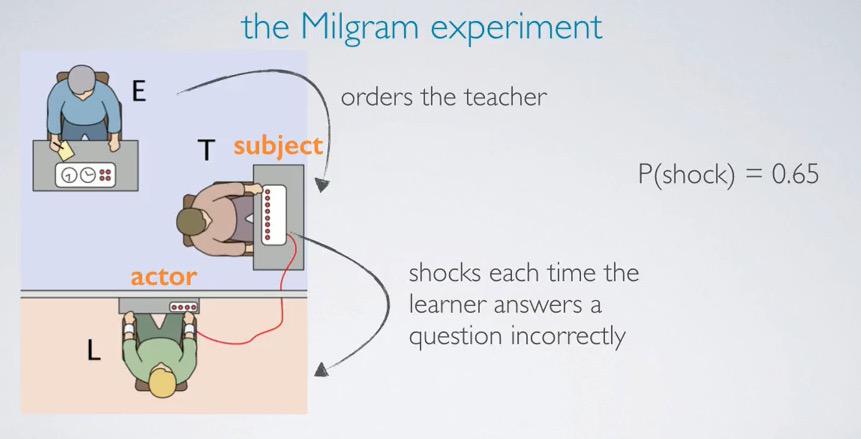
Screenshot taken from Coursera video, 01:15
For explaining more about Binomail, here we will take Milgram Experiment. In this experiment, the Teacher is the subject, which would tell whether the teacher wants to do thing against his conscious. The Experiment will order the teachers to shock the Learner, which actually just sound recorded each time the teacher send a shock. The teacher has 'blinding' about the learner and found that consistently overtime probability of teacher giving shock is 0.65
Each subject of Milgram's experiment is considered as trial.And she/he labeled success if he administer a 'shock' and failure otherwise. In this case the probability of sucess, p = 0.35
When a trial only has two possible outcomes, we call this Bernoulli random variable.
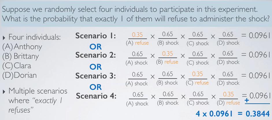
Screenshot taken from Coursera video, 05:29
So when doing the experiment on 4 people, we have possible outcomes of 2^4. But only regarding scenario where exactly 1 person that we concern. This turns out to be 4 scenario that each of the person try.
With all of the scenario simulated, we see that exactly all the probability is the same. Since all the person is independent, we can multiply them directly. Since this is disjoint events of 4 scenario, we can quickly do:
res = P(scenario) * n_scenario
This eventually make a perfect setting for Binomial Distribution.
Screenshot taken from Coursera video, 07:12
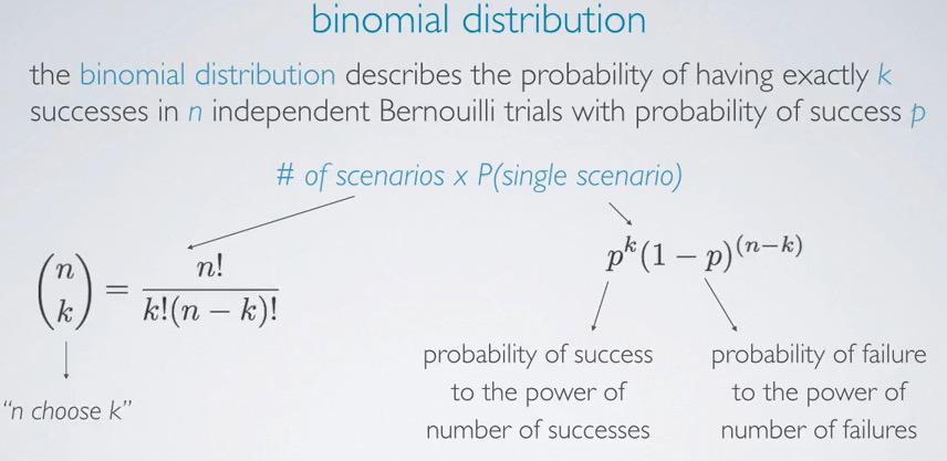
So doing earlier steps by hand would be quiet tedious, as we have to jot down all possible conditions. What we can do is using binomial distribution for our problem.
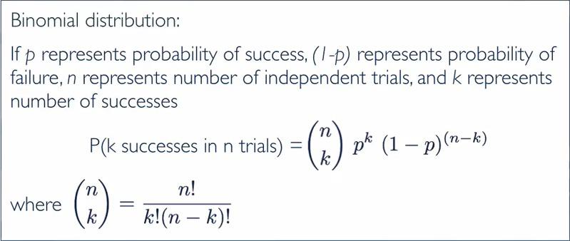
This is the main formula for Binomial Distribution, and as long we have three of the required variables, we can do the calculation.
Screenshot taken from Coursera video, 09:23
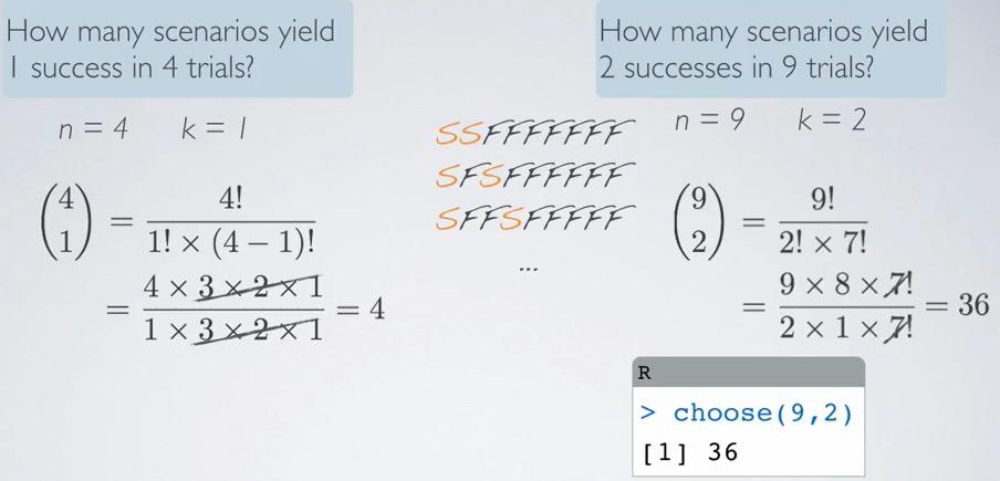
For the first K '4 choose 1' can simply be calculated doing the formula above. For the second one, as we can see at the first three simulated, things can get complicated easily, so we're doing '9 choose 2'.
This can get easily computed in R
%R choose(9,2)
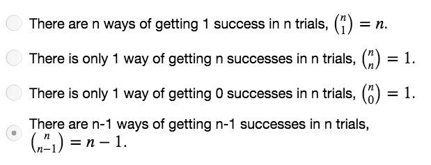
Screenshot taken from Coursera video, 07:12. Only last one is false
%R choose(5,4)
So to put it concretely,
Screenshot taken from Coursera video, 09:53
The conditions for binomial are:
- The trials must be independent
- The number of trials, n, must be fixed
- each trial outcome must be classified as a success or a failure.
- The probability of sucess,p,must be the same for each trial(which is to be expected, agree with number 1)
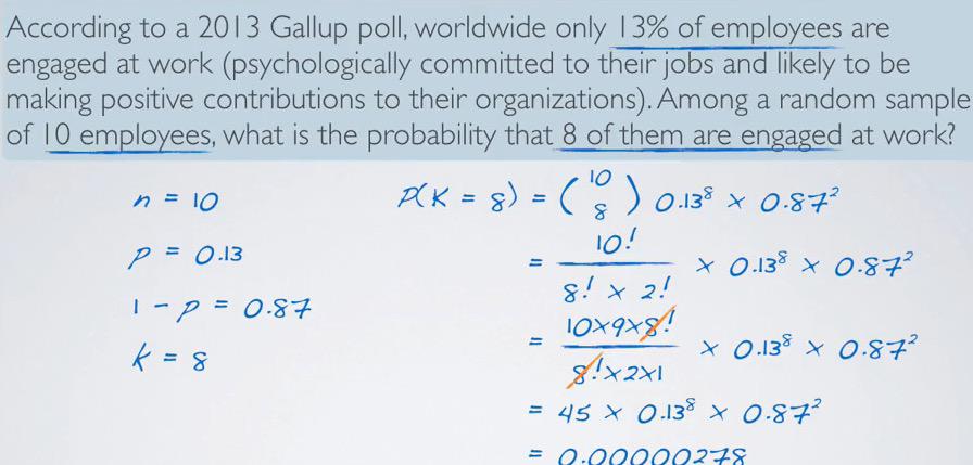
Screenshot taken from Coursera video, 13:43
Pay attention that random sample means we know that the employees, the trials, are independent. And the reason that we're getting very small probability because the power magnitude, we would expect that find probability of success from 10 people is so much lower than the probability of 8 people.
Alternative way of thinking is that, prob sucess is really low, finding 8 in 10 people that succeed, is magnitudely low. Things could go different if we only find 2 success in 10 people, which goes to probability 0.2~0.3.
To do this in R,
#k,n,p
%R dbinom(8,size=10,p=0.13)
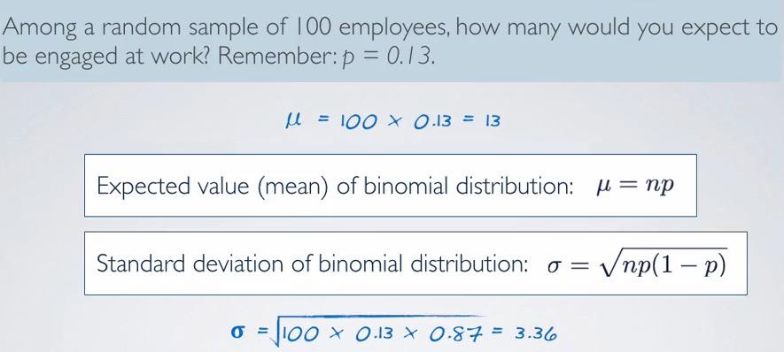
Screenshot taken from Coursera video, 17:13
So doing some simple probabilistic given n samples and probability, we can guess the exact value. And guess the exact value is the expected value in binomial. Standard deviation can also be counted as the following, which in this case give 3.36. So give or take 68% of 100 employees falls in plus minus 3.36. Say, why binomial? Is it the shape because there's only two possible conditions?
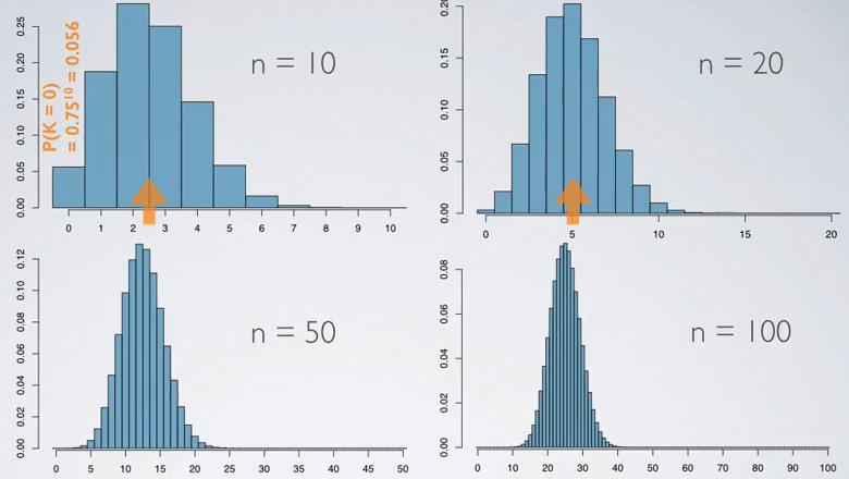
Screenshot taken from Coursera video, 02:14
The binomial will looks closer to the normal distribution as the number of trials increases. This is get by the probability of success, p = 0.25. In the top left distribution, the complement probability, 0.75 is raise to the power of 10(because success case =0). This will give right skewed distribution to be more normal.
Screenshot taken from Coursera video, 03:51
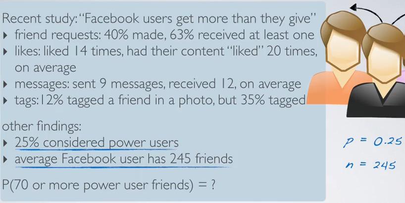
Study found that we actually get more than what we give. The power users is the users in facebook who give more than they get. So we're actually calculating the probability of success, of finding the power users.P(K>= 70)?
Screenshot taken from Coursera video, 07:40
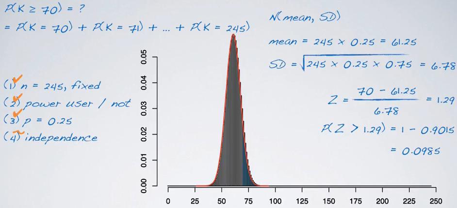
As larger n shape more to normal distribution. We can use the benefit of normal distribution. With binomial, the probability of exact value is the only must condition. So more than probability of success, should be calculated independently like shown in the sample until the number of trials n.
We can calculate this using normal distribution and its properties. Like the formula given earlier, mean can be get from the directly product the number trials and probability of success. Standard deviation from square root of number of trials times probability of success times probability of failure. We can get Z-value and using it to predict the probability.Remember that we want to get the probability of at least 70, so we have to take the complementary probability, since z probability only compute below Z.
In R, this can get by
%R pnorm(70,mean=61.25,sd=6.78,lower.tail =F)
This also can be done using another command of R
Screenshot taken from Coursera video, 09:53
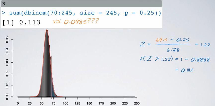
%R sum(dbinom(70:245, size = 245, p=0.25))
So it turns out to be so different than earlier calculations. This can happen in two ways. First it's because the binomial doesn't exactly shape like normal-density function, you can see the bar chart. Second, the 70 of the value is actually cut off and out of the distribution. We can reduce the k by 0.5, and recalculating using R:
%R pnorm(69.5,mean=61.25,sd=6.78,lower.tail =F)
This can also be done by applet : http://bit.ly/dist_calc
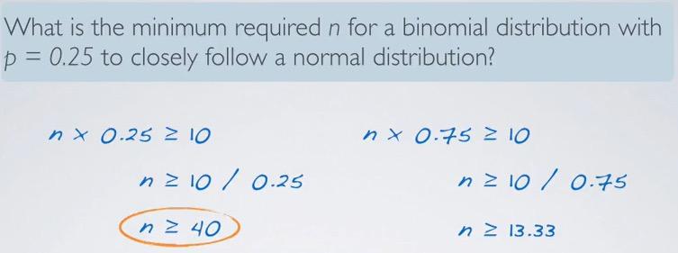
So we know that by taking certain condition that binomial shape like normal distribution, we can take advantage of normal distribution. But if we can't see the distribution? What is the requirement?
Screenshot taken from Coursera video, 12:07
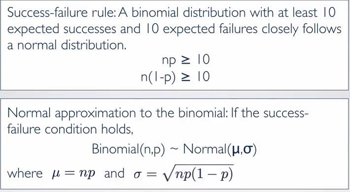
We also have 0.5 point adjustment for k. But what's important here is the sample size, how you're going to be big enough that will somehow shape into normal distribution. Later in statistical inference, there's only two oucome in categorical variable, so it's shape binomial. We can predict the variable as long as binomial shape into normal.
For the formula above we know that we need at least 10 succeses and 10 failures to shape into normal distributions.
Screenshot taken from Coursera video, 14:04
Binomal Examples
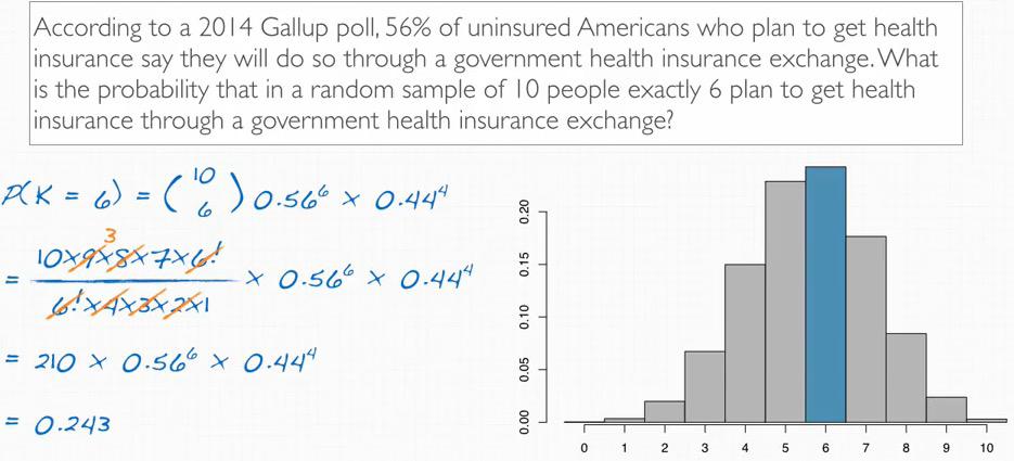
Screenshot taken from Coursera video, 02:58
This can be calculated using R
%R dbinom(6,size=10,p=0.56)
This will get probability that closely approach to the normal distribution. What we expect is actually is(expected number of successes,k):
Expected Value = mean = nxp = 5.6
We expect 5.6 from our calculation, but the histogram prove that 5-6, and 5.6 is not too far behind.
%R dbinom(2,size=10,p=0.56)
Using it in n = 1000 and k = 600, because the Law of the Larger Numbers, makes the probability will be conceptually smaller.
%R dbinom(600,size=1000,p=0.56)
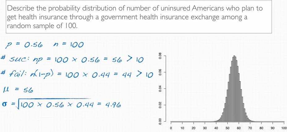
Screenshot taken from Coursera video, 06:29
To describe normal, we need to be exactly sure of the minimum required from the binomial case. When shape like normal, we also need to know mean and standard deviation to plot.
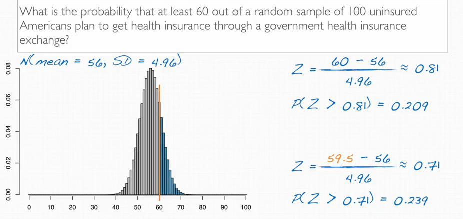
Screenshot taken from Coursera video, 09:59
This can be calculated by applet or dbinom R command. Using z-score, the k value once again has to be decrement by 0.5 because no exact value is 60.
%R pnorm (60-0.5,mean=56,sd=4.96,lower.tail=F)
%R sum(dbinom(60:100,size=100,p=0.56))