A/B Testing Single Metric
When you have single evaluation metric, you have to know what is the impact of your results to the business side. Analytical speaking, you want to find whether your results is significantly different. You then also want to know about the magnitude and direction of your changes.
If your results is statisically significant, then you can interpret the results based on the how you characterize the metric and build intuition from it, just as we have discussed in previous blog. You also want to check the variability of the metric that you experiment.
If your results is not statiscally significant when it really should, then you can do two things. You could subset your experiment by platform, time (day of the week) see what went wrong or different significant if subset by those features. It could lead you to new hypothesis test and understand how your participants reacts. If you just begin in your experiment, you should cross-check your parametric hypothesis and non-parametric hypothesis test.
Effect Size
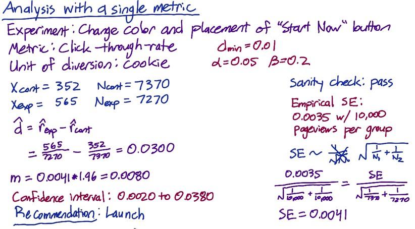
Screenshot taken from Udacity, A/B Testing, Single Metric Example
The next experiment is about change color and placement of "Start Now" button. The metric used is click-through-rate, and the unit of diversion is cookie. There's two things that we can't use analytic standard error. First because our unit of analysis is different than unit of diversion, then the empiric variability and analytical variability expected to be different. Second, more importantly CTR is not following binomial(normal) distribution, instead poisson distribution. The variability can only be calculated empirically.
Assume Audacity have passed the sanity check for the experiments, want to know analyze whether the changes is worth it for business metric (meaning, the results is statistically significant) and have calculated empirical standard errors. To know which standard errors they want, they calculate the sample size and have 10.000 for each group.
After they experiment, they have control and experiment grou, number of clocks and pageviews which summarize as above X(number of clicks), N(number of pageviews). We have 0.0035 as our desired standard error earlier, and normalized by scalling factor:
$$ SE = \frac{SE}{\sqrt{\frac{1}{7370}+\frac{1}{7270}}} $$
Next we build a confidence interval using observed outcome as our point estimate as depicted by the image above. Since we determined that anything outside practical difference 0.01 (dmin) will be significantly different, and indeed the CI is outside of the boundary (typo in the image, CI should be 0.022 to 0.038). So it's recommended to launch the experiment.
Sign Test
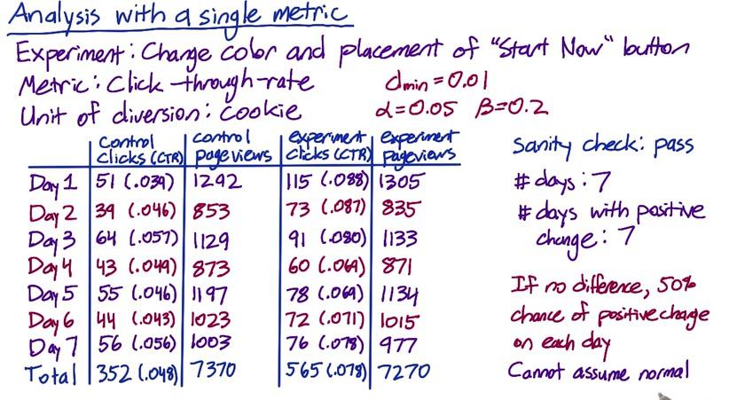
Screenshot taken from Udacity, A/B Testing, Single Metric Example
Next we have another example. Suppose we want to experiment changes which will have positive increase every day. Here we have 7-days experiment. We want to know whether positive increase every day results is so rare due to chance that it could be affected by changes in our experiment. Using binomial distribution is not an option, since number of success and failures needs to be at least 5, and we don't have number of failures.
We can calculate this using binomial:
%R choose(7,7) * 0.5**7 * 0.5**0
The results is 0.0078. But this is only a one-tail p-value. Because we want to find what's significantly different, we multiply it by two to get two-tail yields 0.0156. The results is still statistically significant (above dmin) that we should consider launch the experiment.
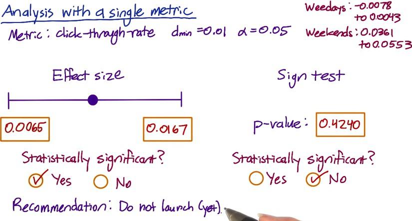
Screenshot taken from Udacity, A/B Testing, Checking Invariant, Part 2
Let's take this to another example and calculate the effect size and sign test.
Xs_cont = [196, 200, 200, 216, 212, 185, 225, 187, 205, 211, 192, 196, 223, 192]
Ns_cont = [2029, 1991, 1951, 1985, 1973, 2021, 2041, 1980, 1951, 1988, 1977, 2019, 2035, 2007]
Xs_exp = [179, 208, 205, 175, 191, 291, 278, 216, 225, 207, 205, 200, 297, 299]
Ns_exp = [1971, 2009, 2049, 2015, 2027, 1979, 1959, 2020, 2049, 2012, 2023, 1981, 1965, 1993]
Xcont = sum(Xs_cont)
Ncont = sum(Ns_cont)
Xexp = sum(Xs_exp)
Nexp = sum(Ns_exp)
import numpy as np
d = float(Xexp)/Nexp - float(Xcont)/Ncont
scaled_factor_anl = (np.sqrt(1./5000+ 1./5000))
scaled_factor_emp = (np.sqrt(1./Ncont+ 1./Nexp))
SE = 0.0062*scaled_factor_emp / scaled_factor_anl
m = 1.96*SE
print 'Confidence Interval = {}'.format((d-m,d+m))
The results we see is that analytically this is significantly different, but notice that the practical positive boundary is within the interval. So we may want to hold that thought, let's see another example.
import pandas as pd
df = pd.DataFrame({'clicks_control':Xs_cont,
                   'pageviews_control':Ns_cont,
                   'clicks_experiment':Xs_exp,
                   'pageviews_experiment':Ns_exp})
ctr_exp = df['clicks_experiment']/df['pageviews_experiment']
ctr_cont = df['clicks_control']/df['pageviews_control']
df['isHigher'] =   ctr_exp > ctr_cont
df.head()
%R sum(dbinom(9:14,size=14,p=0.5)) * 2
Here we see that our p-value is very large that it's not statistically significant. It's a good idea to analyze this, and turns out the CTR is higher on weekends for the experiment vs weekdays. Based on this results, we may not yet launch the experiment, and try to investigate why our experiment doesn't affect weekdays.
Gotchas
Sometimes like earlier in the example, your hypothesis test is not agreeing with sign test. Again, you might want to take a look your data by platform, or any subset of the population. It is a possibility though that both test can yield different results. This is called simpson's paradox. Where you have sub-group that is not statiscally significant, but turns out to be significant when you add them all up together. It's good thing to find out what drives the different, maybe check whether your new user behave differently on weekend and experienced user behave differently on weekdays.
Simpson's Paradox
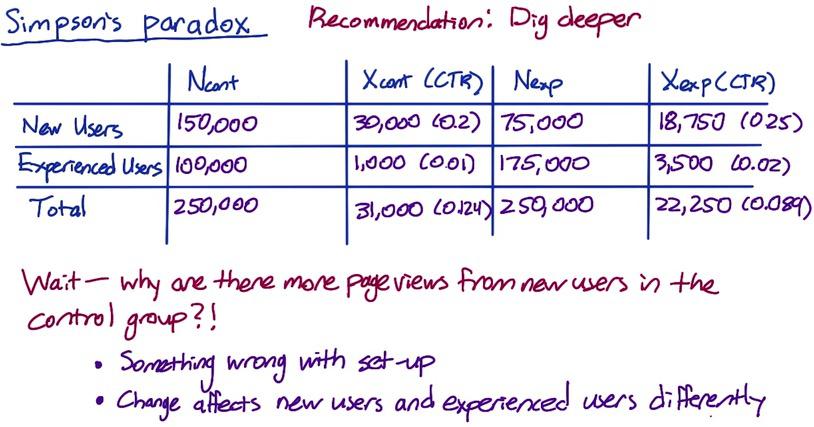
Screenshot taken from Udacity, A/B Testing, Gotchas, Simple Paradox
This is an example of Simpson's Paradox. The experiment is higher in CTR for both groups, but lower overall. This could be because your experiment behave differently for experience and new users, but still make a positive impact.
Earlier, we do sanity check to make sure all users are randomly sampled and have equal proportion. But this is still could happen, either with setup or different experience. This experiment still success but it's a good idea to investigate this to know what's going on otherwise you won't build a valid conclusion.
Disclaimer:
This blog is originally created as an online personal notebook, and the materials are not mine. Take the material as is. If you like this blog and or you think any of the material is a bit misleading and want to learn more, please visit the original sources at reference link below.
References:
- Diane Tang and Carrie Grimes. Udacity