Variability of Metrics
When characterizing our experiment, we're talking about how the metric can used in particular situation. We want to know range of possible condition that metrics can be used, and that's variability. Usually, when we talking about probability (e.g. click-through-probability) or count of users, we can see nice normal distribution by plot it in histogram. This would make it easy for us to use theorically-compute variability, in form of Confidence interval. We could also use our normal practival significance level. However, when using video latencies like in previous blog gives us sort of lumpy shape, we want to compute the variability empirically. This blog discuss about how we characterize metrics for our experiment, specifically by measures of spread.
Screenshot taken from Udacity, A/B Testing, Variability Example
Earlier, we have talked two kinds of variability, one that follows normal distribution can be computed using theoritically-computed confidence interval. The second is that when we see not-so-normal distribution, we use empiric variability. Recall that when using CI, we need to know mean, standard deviation and sample size. And for CI to be true, minimal sample size of 30, or much larget when it's not follow normal distribution when we standardizing.
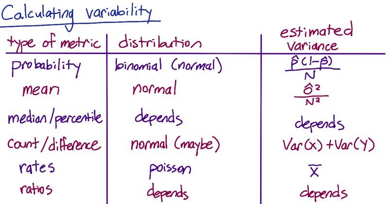
Probability, mean, count/difference follow normal distribution. So it expected that their variance can be computed analytically. But When we use median as point estimate, the variability will not follow normal distribution. And the distribution of ratio will follow distribution of its denominator and enumerator. For poissson distribution, I quoted Udacity's A/B testing from their material:
The difference in two Poisson means is not described by a simple distribution the way the difference in two Binomial probabilities is. If your sample size becomes very large, and your rate is not infinitesimally small, sometimes you can use a Normal confidence interval by the law of large numbers. But usually you have to do something a little more complex. For some options, see here (for a simple summary), here section 9.5 (for a full summary) and here (for one free online calculation). If you have access to some statistical software such as R (free distribution), this is a good time to use it because most programs will have an implementation of these tests you can use.
If you aren’t confident in the Poisson assumption, or if you just want something more practical - and frankly, more common in engineering, see the Empirical Variability section of this lesson, which starts here.
Screenshot taken from Udacity, A/B Testing, Variability Example
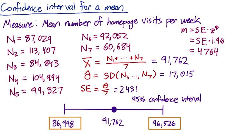
We take mean as summary metrics for measuring number of homepage visits per week. Using mean, we know that its variability can be computed analytically, so we follow the formula as:
import numpy as np

arr = np.array([87029, 113407, 84843, 104994, 99327, 92052, 60684])
x = arr.mean()
sd = arr.std(ddof=1)
se =sd/np.sqrt(arr.shape[0])
me = 1.96 * se
(x-me,x+me)
Non parametrics is useful when you have funnier distribution than normal, that makes it hard using normal summary statistics and CI. When calculating variability like in the table above, we don't expect normal distribution. It's computationally expensive but also useful. If there's changes in our data in midway that larger than chance, we can use non-parametrics, though we don't now the size. If we make positive changes, and compute the variance of the changes in the data, look at the distribution. If it normal, use normal summary statistic and CI. If it funnier, use non-parametric.
At this point, we agree if we have simple normal distribution, we can use our usual metric. But when the distribution is funnier, often due to largely complex system, we choose empirical variability. But often we can't use empirical, because it's underestimate the changes. One alternative is using A/A testing.
A/A testing differs from A/B testing. in the sense that A/B is for A(control) and B(experiment), we want to detect changes that we care about, A/A testing is for control vs control groups. We want to identify changes that we don't know (lurking variables) that makes variability of our data.
A/A usually required to have larger sample size, as we now standard deviation (SE) minimized by quadratical increase of our sample size. This is tends to be expensive, gathering sample size. The alternative to this is using one big experiment or bootstrapping, chunking into smaller part and use an experiment on that. We don't always use bootstrap if it doesn't agree with our analytical variance. We have to use big experiment instead. But if it does, we can safely move on.
Empiric variability is an observation with little calculation using A/A tests. With A/A tests, we can do three things:
- Compare results from analytical and empirical (sanity check)
- Estimate variance and calculate CI
- Directly estimate CI result test
Screenshot taken from Udacity, A/B Testing, Variability Example
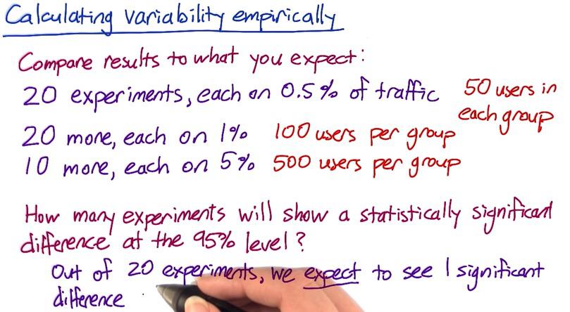
Suppose we want to compare results, divided by these experiments. Analytically out of 20 experiments, you should see 1 significance difference (Out of 20 CI, one interval won't captured significance different). We can verify this empirically.
We can do two other things for sanity checking our empiric variability as mentioned.
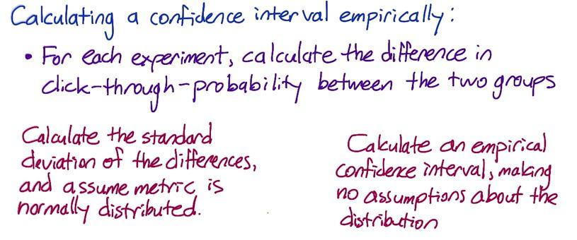
You can estimate variance empirically and calculate CI if you can't use analyticalically. In the example, we know that our difference betweeen A/A testing both groups. We can calculate standard deviation on the diffrence, and used this as opposed to analytical standard of error. One advantage of using empiric, is that the standard deviation can be used across experiments. If we do this by analytical, we know standard error will be based on the size of the data, which will be vary across size of the experiments.
Screenshot taken from Udacity, A/B Testing, Empirical Confidence Interval
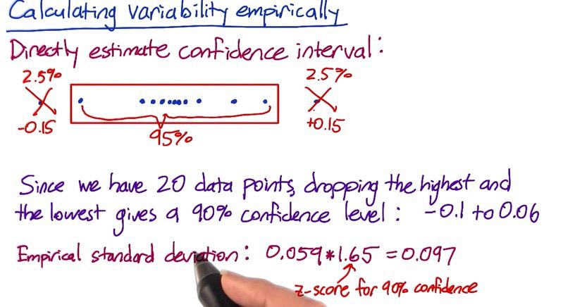
Finally, we can directly estimate CI result and validate with our empiric standard deviation, if you don't expect normal distribution.
Suppose we have 95% CI and we want to cut off our largest and smallest data points in the interval (20 points in 100% ratio, decrease 5% by cutoff two points). This will gives us 90% interval which range from -0.1 to 0.06. Using our SD empiric, multiply by 1.65(z-score 90%), we got to highest 0.097. It's quite difference than empiric, but it's contributed by two other factors. The fact that 20 is too small (recall 30 sample size for at least normal), which we have to increase our sample, if it doesn't took you enough time.
Bootstrapping
Using bootstrapping, we can simulated many experiments when we actually use one big experiments. Suppose we have one experiment. This experiment is used to test many changes that we make, and see what actually make significant difference. First we divided our sample into two group, control and experiment group. Then for every experiment, we random sampled from each side of the group, run it as simulated experiment. We random sampled experiments from pool sample that's actually one experiment. Bootstrap is particulary useful because we can take as many sample as we can, with replacement, from limited sample. Bootstrap is other technique that can be used aside from A/A tests. You can calculate CTP from 40 A/A tests, or 40 bootstrap samples. Please check my other blog to see some explanation with boostrapping.
a = """0.02
0.11
0.14
0.05
0.09
0.11
0.09
0.1
0.14
0.08
0.09
0.08
0.09
0.08
0.12
0.09
0.16
0.11
0.12
0.11
0.06
0.11
0.13
0.1
0.08
0.14
0.1
0.08
0.12
0.09
0.14
0.1
0.08
0.08
0.07
0.13
0.11
0.08
0.1
0.11"""


b = """0.07
0.11
0.05
0.07
0.1
0.07
0.1
0.1
0.12
0.14
0.04
0.07
0.07
0.06
0.15
0.09
0.12
0.1
0.08
0.09
0.08
0.08
0.14
0.09
0.1
0.08
0.08
0.09
0.08
0.11
0.11
0.1
0.14
0.1
0.08
0.05
0.19
0.11
0.08
0.13"""
Supppose wee have one big experiment, the sample size for both groups are 100. We take A/A test and random sampling for 40 experiments.
arr_a = np.array(a.split('\n'),dtype='float32')
arr_b = np.array(b.split('\n'),dtype='float32')
a_sim = np.random.choice(arr_a,size=100)
b_sim = np.random.choice(arr_b,size=100)
Screenshot taken from Udacity, A/B Testing, Empirical Variability, Bootstrapping
We want to sanity check both techniques, by first using empiric standard deviation, and second using empiric confidence interval.
using empiric standard deviation, and calculate 95% CI
diff = (arr_a - arr_b)
avg_diff = diff.mean()
std_diff = diff.std()
ME = 1.96*std_diff
(avg_diff-ME,avg_diff+ME)
Empiric confidence interval
#40 data points, 95% CI can be gained by subtracting 2 points at max and min (because CI two-tailed)
diff.sort()
diff2 = diff[1:-1]
(diff2.min(),diff2.max())
The difference between two method can be minimum, if we have more than 40 sample size. Since we don't expect normal distribution, it could be not normal at all, so greater sample size require to make more normal difference in distribution.
In summary, empiric and analytic can be two techinique to validate your result. For first measurement, you want to use analytical. It's often useful and work for simple experiment. As you add more complexity to the system, like running many experiment, empiric can be a good choice. There's some metric that favor empiric more than analytical. There's also some discrepancy occurs between both technique, but it's often practically neligible. You want to validate the variability by using empirically, and analytically. We will discuss this in next blog.
Disclaimer:
This blog is originally created as an online personal notebook, and the materials are not mine. Take the material as is. If you like this blog and or you think any of the material is a bit misleading and want to learn more, please visit the original sources at reference link below.
References:
- Diane Tang and Carrie Grimes. Udacity